Revised:
Expo provides powerful functions for analyzing data both during and after an experimental run. This section describes Expo's self-contained analysis routines. If you want to undertake your analysis externally, Expo can export data as an XML document that can be read by another programs. Appendix F describes a suite of routines for Matlab that analyze the data in XML documents.
Analysis functions are all accessible through a single analysis window that you open by first bringing to the front the program whose data you want, then choosing Data->Examine (Command-E). You can also open an analysis window for any loaded data file by choosing the file's name from the Data->Loaded submenu, or by double-cliking the file's Status window.
The table in the lower part of the window provides what is essentially a spreadsheet through which you can manage the analysis. Each row in the table represents a single slot in the schedule (if a slot controls a matrix of substates the whole matrix is unfolded as if each substate occupied a separate slot). The first column in each row shows the number of times that slot was run. The second column shows the name of the state (or matrix substate) controlled by that slot. If you pass the cursor across any cells in the first two columns, Expo will display, in the box above the table, a list of the routines in the state. Cells in subsequent columns are available for you to enter formulas for analyzing data collected by the state in the slot.
Each cell can contain one of four kinds of formula:
1. A formula to analyze state events.
2. A formula to analyze the spike train.
3. A formula to analyze any continuously sampled analog signals.
4. An expression that manipulates results displayed in other cells.
The results of the analysis specified in a cell can be a single value, or an array of values. In either case, Expo can display and print graphs relating values (or arrays of values) in different cells, and it can display and print tables. Graphs and tables can be copied to the clipboard and pasted into documents managed by other applications.
Expo can also fit curves to the results of analysis, and can add the curves to any graphical display of data.
A formula specifies a class of event (spikes, analog signals, state events) and an analysis to be undertaken on it, or is an expression relating results held in other cells. Click the tab to choose the type of analysis (State Event, Spike, Analog Signal, Expression linking cells) you want. Each tab displays options for setting the appropriate analysis formulas. (If no spike events or no analog signals have been collected, no tabs are provided for them.)
To enter a formula in a column of cells, click the column header to select the cells. You may enter a formula only when a single column is selected.
You can undertake the usual editing operations (cut, copy, paste, delete, with undo) on columns of formulas. To clear formulas, select the relevant columns, then choose Edit->Clear.
A new analysis table starts with 7 columns in which you can enter formulas. You can add and remove columns and can rearrange them within the table as needed. To append a column click Append Column. To remove a column select it then click Remove Column. To move a column to a new position drag its header to the required spot.
By default, Expo enters a formula in every cell in a column. You can prevent formula entry in specified rows by masking them. To mask a row (or rows) select them by clicking in either of the two left most columns, then Control-click to display the context menu. Choose Set Row Mask. Expo displays a pale pink background on cells in any row that is masked.
When a row is masked, Expo will never enter a formula in any of its cells. If you mask the row after having entered a formula, Expo will use the formula as usual in analyzing data, but will never make its results available for other operations, such as plotting graphs, or fitting curves.
You can clear individual row masks by selecting the rows and choosing Clear Row Mask from the contextual menu. You can clear all row masks (without need to select rows) by choosing Clear All Masks.
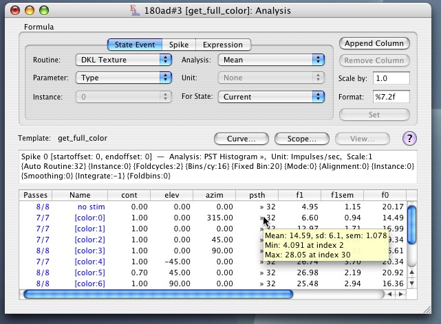
When you analyze state events, the formula in each cell operates on the value of a single parameter in a routine. Choose the routine from the Routine pop-up menu, and the parameter from the Parameter pop-up menu. The Routine menu identifies all the routines called in the program. Since a single routine may be called more than once within a state, and have different values for its parameters, you may also need to choose from the Instance pop-up menu the occurrence you want (0 being the first).
In the right-hand side of the tab, choose from the Analysis pop-up menu the kind of analysis you want undertaken on the routine parameter. The different analyses are described in Analysis Routines. An analysis can result in a single value or an array of values. When an analysis yields an array result, its name appears in the menu with the character » appended to it; for a two-dimensional array, a second » is appended. Each item in the menu refers to an analysis that will, by default, use data recorded on all passes of the running program through the slot/state. For example, the Array » analysis will yield an array of the values of the parameter recorded on every pass of the program through the slot/state. The section Scope of Analysis explains how you can restrict the scope of analysis to a subset of the passes.
| An analysis with a bullet before its name (•Count, •Times, •Pass Indexes) provides the same information regardless of which Routine and Parameter you have chosen for analysis. |
Normally you will want the formula in each cell to analyze data for the state represented by the table row that contains the cell. On occasion you might want an analysis to work with parameter values in the state run just before or after the represented one: you might want to know about the parameters of a persisting routine from an earlier state or, if a stimulus condition is set by one state and a psychophysical response is collected in the one run immediately afterwards, you might want the response to be linked to the stimulus condition. You can choose whether the analysis is to be undertaken on data collected by the state represented by the table row in which the formula is set, or on data collected by a state run before or after the one represented (the "current" state). Choose this from the "For State" pop-up menu. The default setting is to analyze data for the current state.
To set a formula, click Set. Some analysis formulas require auxiliary parameters. If you have set one that does, Expo will display a sheet asking for additional input before proceeding. Expo loads the formula into every selected cell, then runs the analysis and displays the result.
If a result is a one-dimensional array of values, Expo will display » in the cell, together with the size of the array; if the array is two-dimensional, Expo will display »». When the cursor rests over a cell that has an array result Expo will display a tooltip window containing summary statistics for the array (see figure above); you can display the whole array expanded in a menu by Control-clicking the cell. You can also view arrays as tables, or graphs, on which more below.
| If the event queue contains no data of the kind required by a formula, or some analysis error occurs, Expo will display ?? in the cell. |
When you place the cursor over any cell with a formula, Expo will display a description of the formula in the box above the table.
To change the formula in a column that already contains one, select the column, choose the new analysis, and click Set.
The results of many analyses can be expressed in more than one unit (e.g., radians or degrees). Use the Unit pop-up menu to choose the units in which you want the results expressed.
You can have the results scaled by any constant (except 0). To change the default scale (1), enter a constant in the Scale by box to the right of the tab.
By default, Expo displays results to two decimal places, but you can change this to suit your needs. Use the Format box to specify the format and precision with which results will be displayed. Enter a format specifier of the kind you would use with the C function printf.
| Expo uses the current settings of Unit, Scale and Format when it builds a formula, so if you want to use other than the default settings, be sure to organize them before you set the formula. |
On the spike tab choose from the Spike pop-up menu the spike you want to deal with. Each spike is identified by its template and channel on which it was recorded; if only one spike was recorded, the menu is dimmed. Choose from the Analysis pop-up menu the analysis you want undertaken on the spike train. The different analyses are described fully in Analysis Routines. When an analysis yields an array result, its name appears in the menu with » appended to it (»» signifies a two-dimensional array). Each option in the menu refers to an analysis that will, by default, use the spike times collected during every pass of the running program through the slot/state. For example, the option Count (µ) will calculate the number of spikes collected during the execution of the state, averaged over all passes.
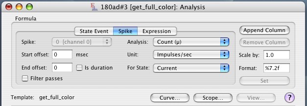
By default spikes are analyzed for the duration of the state represented by the table row that contains a formula. To analyze spikes collected during a state run before or after the represented one, choose this from the "For State" pop-up menu. Beyond specifying the state from which spikes are to be analyzed, you can set the span over which the analysis takes place (covering a fraction of the state, or extending backwards or forwards through the preceding or succeeding pass). To change the time at which the analysis begins in relation to the start of the state, enter a value for Start offset (this can be positive or negative). To change the time at which the analysis ends in relation to the end of the state, enter a value for End offset (this too can be negative or positive). Instead of specifying an end offset you can specify a span duration from the start. Check Is duration to make Expo interpret the End offset value as a duration.
| In setting a span you might specify times at which no data were collected. Expo will analyze data only for passes whose spans fall entirely within the time for which the program was active. This may result in fewer than expected passes being analyzed. If Expo finds no data available for the span requested, it does not deliver a result, and the relevant cell in the analysis table will contain ?? |
If you check Filter passes Expo will apply a filter to restrict the analysis to signals accumulated from selected passes through a state. For more information see the later discussion of Conditional Analysis.
To set a formula in the selected column, click Set. Depending on the analysis chosen, Expo will immediately set the formula and display the result, or will drop a sheet asking you to provide values for some auxiliary parameters. Sheets appear with default settings for auxiliary parameters. When you change settings, these becomes new defaults for your current session.
The Unit, Scale by and Format options work for spikes exactly as they do for state events.
| Some analyses undertaken on spikes, such as FT Amplitude (PSTH), compute frequency components of the spike train. They can be computed only if the state is active for long enough to include at least one period of the relevant frequency. If an analysis cannot be undertaken on the data Expo will display ?? in the relevant table cell. |
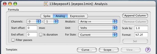
Use the Channels pop-up menus to identify the first and last channels whose signals you want analyzed (if you specify a first channel number higher than the last channel, Expo will treat them as reversed, and correct them when it uses the settings). Channel numbers do not refer to the hardware channel numbers, but to the first, second, etc. whose values were recorded. In the right-hand side of the tab, choose from the Analysis pop-up menu the kind of analysis you want undertaken The different analyses are described fully in Analysis Routines. When an analysis yields an array result, its name appears in the menu with » (one dimension) or »» (two dimensions) appended to it. Each option in the menu refers to an analysis that will, by default, use the signals collected during every pass of the running program through the slot/state. For example, the option Array »» will build arrays containing the waveforms sampled through each channel during the execution of the state, averaged over all passes.
By default signals are analyzed for the duration of the state represented by the table row that contains a formula. To analyze signals collected during a state run before or after the represented one, choose this from the "For State" pop-up menu. Beyond specifying the state from which signals are to be analyzed, you can alter the span over which the analysis takes place (covering a fraction of the state, or extending backwards or forwards through the preceding or succeeding pass). To change the time at which the analysis begins in relation to the start of the state, enter a value for Start offset (this can be positive or negative). To change the time at which the analysis ends in relation to the end of the state, enter a value for End offset (this too can be negative or positive). Instead of specifying an end offset you can specify a span duration from the start. Check Is duration to make Expo interpret the End offset value as a duration.
| In setting a span you might specify times at which no data were collected. Expo will analyze data only for passes whose spans fall entirely within the time for which the program was active. This may result in fewer than expected passes being analyzed. If Expo finds no data available for the span requested, it does not deliver a result, and the relevant cell in the analysis table will contain ?? |
If you check Filter passes Expo will apply a filter to restrict the analysis to signals accumulated from selected passes through a state. For more information see the later discussion of Conditional Analysis.
To set an analysis formula in the selected cell or cells, click Set. Depending on the analysis chosen, Expo will immediately set the formula in the cells) or will display a sheet asking you to provide values for some auxiliary parameters. Sheets appear with default settings for auxiliary parameters. When you change settings, these becomes new defaults for your current session.
The Unit, Scale by and Format options work for analog signals exactly as they do for state events.
You can enter in any cell an expression to perform common arithmetic operations on results computed in other cells.
To create an expression, click the Expression tab and type the expression in the text box. An expression has the following general form:
cell op cell or cell op constant
where cell identifies the column and row coordinates of a cell, constant is a numerical constant, and op identifies the operator. A cell reference consists of an absolute column specification (a letter A through Z) followed optionally by zero-based row number. If no row is specified, the row reference is implicitly the current row. Thus D15 refers to the cell in the fourth column and the sixteenth row; D refers to the cell in the fourth column and current row.
| If you move a column in the table Expo adjusts any expressions in that refer to its cells; if you remove a column, Expo invalidates expressions that refer to its cells. |
In expressions you can use the arithmetic operators
+ – * ÷
the logical operators
= > <
and the function operators
? #
The result of a logical operation is 1 or 0.
The conditional operator ? sets the result to the first operand if the second operand is TRUE, otherwise to NAN.
The operator # works only with arrays, and transforms an array in one of two ways. When used in an expression of the form A#n, where A is an array and n is a scalar value, it forms a histogram of the values in A (excluding nans), distributed over n bins. If n is 0, then the number of bins in the histogram is the number of unique values in the array. If n is invalid (< 0 or greater than the number of input values) it is assumed to be equal to the number of input values. If the expression has the form A#b, where A is an array and b is an array, the result is an array of values that reflects the following transformation: values from the first operand are accumulated in bins determined by their counterpart values in the second operand, the average of each bin is calculated, and the array of bins is ordered by the values in the second operand. For example, if column A is an array of spike counts, and column b an array of contrast values, some of which are repeated, the expression A#b will deliver an array of average spike counts ordered by the contrasts that gave rise to them. The expression b#b would deliver an ordered packed array of contrast values.
Expressions are evaluated left to right and all operators have equal precedence. You can force evaluation order by enclosing an expression in parentheses, and you can nest expressions, to any depth, e.g.
((B0+C)*(5+C4))+D
You can use the unary minus before any element or expression, e.g.,
–C1
Cells to which an expression refers may contain formulas that yield single-valued results or arrays. If any referents yield array results, the result of the expression will be an array of the size of the first array encountered in evaluating the expression.
When writing expressions you need not leave white space between elements. Cells to which an expression refers may contain formulas to analyze spikes, analog signals, or state events, or may contain expressions.
| When analyzing data Expo makes two passes through each cell in the table. It works through cells in a row from left-to-right, and through rows from top-to-bottom. Expo will not evaluate an expression that makes more than one level of forward reference to other expressions. |
Click Set to enter a completed expression in the cells of the selected column. Before entering the expression Expo checks the syntax, and also that no references are to non-existent cells.
All cell references in an expression are absolute; when you cut or copy, then paste the contents of cells that contain expressions, Expo does not adjust any references in the expressions.
The Scale by and Format options work for expressions exactly as they do for state events.
You can recover the text of an expression already entered in a cell by Option-clicking the cell.
You can at any time change the formula in a column of cells by setting up the type of formula you want, then selecting the column and clicking Set. To base a formula or expression on one that is already installed in a cell, you can quickly build the appropriate menu settings and the scale and format settings by Option-clicking the column.
Editing operations such as copy or paste, on cells that contain results, carry formulas and results. If you paste cell contents anywhere other than into an analysis table, only the results are pasted, as text.
By default, Expo will analyze events in the spike, analog or state event queues for every pass through the relevant slot/state. You can restrict the analysis to data collected during a subset of the passes.
Specify the scope of the analysis by clicking Scope…. Expo will display a sheet in which you can specify the first pass through the slot/state for which you want to examine data, the last pass you want examined, and the steps between. By default, data for every pass are analyzed, represented by a starting pass of 0, a finishing pass of –1, and a step of 1. Negative pass numbers denote "from the end," with –1 meaning "the last pass." To analyze data collected during the last three passes, you would therefore enter a starting pass of –3 and a finishing pass of –1. If you specify starting or finishing passes outside the range for which data have been collected, Expo will analyze no data, and display ?? as the result. To analyze data for a single pass, enter the same number for both starting and ending passes. A step of 1 means examine data for each successive pass, a step of 2 means every other pass, etc.
The scope you specify is an attribute of the table, not of a particular cell, and so applies to every cell. When you define a scope, Expo recalculates results for all cells.
When you have set a scope that is less than all passes, Expo will indicate this in the first table column.
When you open a new analysis window, Expo creates a table row for every slot/state in the schedule, with matrix substates unfolded. The order of unfolding is from outermost dimension to innermost. If you want to examine data with dimensions ordered differently (this can be useful in controlling how graphs are constructed), or from just specified dimensions or parts of dimensions, you can change the order in which dimensions are unfolded, and you can hide data from parts of the matrix you don't want to see. To determine what is displayed click View… (the button is dimmed if no matrix was run, or the matrix has only one dimension). Expo will display a sheet like this.
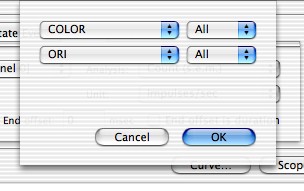
On the left are popup menus from which you choose the order in which dimensions are unfolded. The top menu represents the outermost displayed dimension, the bottom menu the innermost. For each dimension there is a counterpart menu containing a list of the substates on that dimension, plus an item "All". Use this menu to set whether the table should show all substates on that dimension or just the substate at the position specified.
For the purposes of plotting or tabulating results, parts of a matrix that are hidden are treated as though they did not exist.
Expo normally analyzes data collected from all passes through a each state or matrix substate (subject to the scope settings), but you can also restrict the analyses at two levels: you can examine only passes in which the state or substate of interest immediately preceded or followed a specified state or a range of matrix substates, and (for spikes and analog signals) you can set the formulas in individual table cells to select passes according to the results contained in partner cells.
To set up a contingent analysis for any row in the analysis table, select the row, then Control-click either of the two left-hand columns. You can set conditions on multiple rows in a single operation by selecting several rows. From the context menu choose Set Condition…. Expo will display the following sheet.
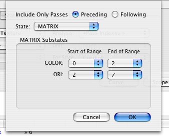
Click the Preceding or Following button to choose whether the passes to be analyzed will depend on the preceding state or the succeeding one. Choose from the popup menu the preceding or succeeding state that will determine which passes are analyzed. If you choose MATRIX, you can specify (via the popup menus in the box) the range of substates that must precede or succeed any acceptable pass.
If you have imposed a contingency on the analysis for a particular row, Expo will display § in the first cell, beside the count of passes analyzed.
When setting a formula to analyze spikes or analog signals you can specify a filter that will select the passes used in the analysis. The cell's filter is applied in addition to any contingent analysis specified for a row (above). If you check Filter passes in the Spike or Analog tab, and the table cell immediately to the left of the one in which you are setting the formula contains an array, Expo will include in the analysis only data from passes in which the corresponding array element was neither zero nor NAN.
If the filter array is the result of an expression, the expression should not make forward references to other table cells.
| Expo will silently ignore the Filter passes setting if you are setting a formula in the first column of the table, or if the table cells that would provide filters do not contain arrays. If a filter array contains fewer elements than the number of passes being analyzed, passes for which there is no corresponding filter element are excluded from the analysis. |
When a cell contains a filtered result Expo indicates this by displaying in the cell (after a | ) the number of passes from which the result was calculated.
You can save the collection of formulas contained in a table and use it as a template for subsequent analyses. A template contains all the information about formulas and masks, but does not contain information about the scope of the data analysis, or curve-fitting settings.
To save a template, make sure the main analysis window is active, and choose File->Save (or Save As…). Since the template will also contain the titles of columns, you should ensure before saving the file that these are set to the names you want. You can give a template any name you want, but for reasons noted below there is real benefit in giving it the name of the program that gave rise to the data being analyzed. A saved template contains information about all cells in a table, even those for parts of a matrix that are hidden from view.
Opening and Using Saved Templates
To open and load any saved template choose File->Open….
All loaded templates are accessible through the Data->Template submenu (a template can be chosen only when the main analysis window is active). A template can be used on a data set only if the template has at least as many rows as the data set. By default Expo dims items for any templates that do not have exactly the same number of rows as the data set. You can relax this constraint, and permit the use of templates with more rows than the data set by choosing Expo->Preferences and checking Enable Oversize Templates.
To apply a template to the current set of data, choose from the Template submenu. Expo will apply the template and analyze data for all cells that have formulas. The template's name appears immediately above the table.
To use another template in the analysis window, simply choose it; after checking whether you want to save any changes to the current template, Expo will clear the existing contents and rebuild the table per the new template.
To replace any template in use with a new blank one, choose New Template from the submenu.
| If a template designed to analyze data collected by a particular program has the same name as the program, Expo will apply the template automatically whenever you open a new analysis window for data collected by the program. (For this to happen the template must be loaded and available in the Data->Template submenu). |
Expo can display analyzed data in graphs. You can view and work with data in single or multiple graphs.
To make any graph you must first select in the table the data you want to display. Expo handles single-valued results (scalars) and array results differently, and the discussion that follows assumes that cells contain single values. Plotting Array Data describes the how Expo handles arrays.
In making graphs Expo treats columns of selected data as X and Y arrays; for a simple XY plot you would select two columns (the left one is taken to be X). To plot the selected data, choose Data->Graph (Command-G). Expo will open a window with the orientation and aspect ratio of the paper used in the printer, and will plot the graph, with axes automatically scaled. Expo calculates the scales by examining the range of data to be plotted, and by default scales X- and Y-axes independently.
In plotting a graph of selected results, Expo never uses data from cells in table rows that are masked.
When you change the size of the window, Expo by default preserves the X/Y aspect ratio. You can relax this constraint via Data->Graph Options….
You can print the contents of the graph window, and you can copy them to the clipboard (as a PDF image). You can save the contents as a PDF file.
Expo allows one Graph window for each data set being analyzed. If you activate the analysis window and select and plot new data, the new graph will replace any currently displayed in the Graph window.
If the data permit (i.e., none have zero or negative values) you can plot data against logarithmic axes. To do this control-click inside any graph and choose Log X Axis or Log Y Axis from the contextual menu. These items are dimmed if the data are not displayable on logarithmic axes. You can set the default axis type via Data->Graph Options….
| If multiple graphs are displayed in the window, all must have the same axis types. If you change the axes on one graph, axes of all others are transformed too. |
Inside a graph the cursor is a cross, and as you move this over the plot Expo displays its co-ordinates (in units of the data plotted) above the graph. You can freeze the display of any co-ordinate by clicking on the point. Click again to release the display.
To identify the row in the data analysis table from which a particular point on the graph was derived, Option-click on the point. Expo will highlight the relevant row in the analysis table with a green background.
Certain kinds of analyses yield values that Expo can interpret as error bars when it plots graphs. By default Expo plots a data column as error bars if the analysis type provides an error measure (variance, s.d., or s.e.m.). You can change this behavior via Data->Graph Options…. To use a column as a source of error values it must be the next selected column after the column of Y values to which it belongs.
You can plot discontinuous selections (Expo ignores unselected columns), so columns of data need not be adjacent. Within a column Expo plots all rows that contain a result, unless a row has been masked.
You can plot multiple selected columns concurrently, on the same graph or different graphs. With its default settings of graph options (which you can change via Data->Graph Options…), Expo behaves as follows:
1. If a single column of data are selected Expo assumes these to be the Y-values, and generates an ordinal set of X-values, starting with 0. If two columns are selected, and the second column can be interpreted as error data, Expo treats them in the same way. Otherwise, the first column is taken as X-values and the second as Y-values.
2. If more than two columns of data are selected the leftmost is treated as the set of X-values, those beyond the second are treated as Y values (or paired Y-values and error values) as appropriate. All sets of Y/error values appear on the same graph. To change the display so that each set of Y/error values occupies its own graph, control-click inside any graph and choose Separate Graphs from the contextual menu. If all the data represent Y (or error) values, you can make Expo display them against an implicit X-Axis by control-clicking inside any graph and choosing Implict X-Axis from the contextual menu.
By default, Expo treats array data as follows:
1. If you select only one column the data in each cell are assumed to represent Y-values, and Expo generates a corresponding array of X-values, starting with 0.
2. If you select multiple columns, Expo generates an implicit X-axis, and selected columns are assumed to contain Y-arrays (or pairs of Y/error arrays if the appropriate column contains error values). Each Y array (or pair of Y/error arrays) in a single row is plotted on its own graph, and a new set of graphs is made for each selected row in the table. You can change these behaviors via Data->Graph Options… and you canoverride them for an individual graph by control-clicking inside it, and choosing from the contextual menu.
3. When the selected data will yield multiple graphs, Expo scales the X- and/or Y- axes consistently across all graphs. You can change this behavior via Data->Graph Options….
4. If arrays are very large (thousands of data values) Expo will subsample them to improve plotting speed. You can change this behavior via Data->Graph Options….
Two-Dimensional Arrays
If the result of an analysis is a two-dimensional array, by default XY plots contain a separate trace for each index on the first dimension (each trace is colored distinctively). If you prefer to see the array unfolded as a single trace, choose Data->Graph Options…, and uncheck New Trace for Each Dimension.
When it makes sense to do so, Expo will display a two-dimensional array as a raster plot. Expo currently does this only for arrays that result from analyzing spike times. To disable this, choose Data->Graph Options…, and uncheck Display as Raster when Possible.
When it makes sense to do so, Expo will display the elements of a two-dimensional array as matrix of normalized grayscale values. Expo currently does this only for arrays that result from reverse correlation. When you pass the cursor over the displayed matrix Expo shows the value of the corresponding array element. To disable this, choose Data->Graph Options…, and uncheck Display as Matrix when Possible.
To configure Expo's graphing, choose Data->Graph Options…
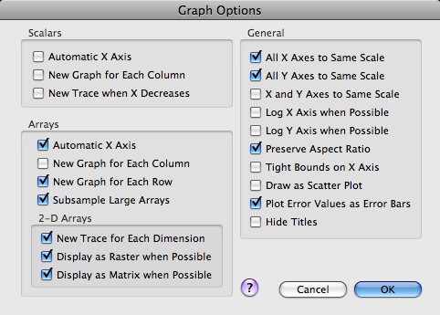
When Expo creates several graphs from selected data, it will force all their X- and Y-axes to the same scale if you check All X Axes to Same Scale and All Y Axes to Same Scale. To force X- and Y-axes to the same scale check X and Y Axes to Same Scale.
The graph window can be resized. Check Preserve Aspect Ratio to ensure that the X- and Y-axes are scaled proportionately during resizing.
Expo automatically scales graph axes appropriately for data, and in doing so sets axis limits to natural boundaries. To force it to place tight bounds on the range of an abscissa, check Tight Bounds on X Axis.
Graphs are plotted with logarithmic X- and/or Y-axes, depending on the setting of Log … Axis when Possible. Expo will not use a logarithmic axis if any value on that axis would be < 0. When a graph is displayed you can change the types of its axes by Control-clicking within the graph.
Data values that represent error quantities (variance, s.d., s.e.m.) are plotted as error bars or as Y values according to the setting of Plot Error Values as Error Bars.
Expo normally connects points by lines (and does not display the points). To show points only, check Draw as Scatter Plot. When a graph is displayed you can change the type of plot (scatter or line) by Control-clicking within the graph.
Expo normally displays a title on each graph. To hide the title check Hide Titles.
For simple graphs of scalar quantities, Expo will provide an automatic (ordinal) X axis if you check Automatic X Axis.
To have multiple columns of Y data plotted in separate graphs rather than as separate traces on a single graph, check New Graph for Each Column.
Multiple sets of data might be contained within a single column. If the X-values within a set increase monotonically (and decrease at the start of each new set) Expo will recognize this and start a new trace on each X reversal if you check New Trace when X Decreases. If there is a reversal after the very first row of data, Expo will treat the Y value in the first row as a special baseline, and draw it as a horizontal trace.
Expo will always provide an automatic (ordinal) X axis if you check "Automatic X Axis".
To have multiple columns of Y data plotted in separate graphs rather than as separate traces on a single graph, check New Graph for Each Column.
To have each row of data plotted in a separate graph rather than as separate traces on a single graph, check New Graph for Each Row.
Plotting large arrays can take considerable time, and their points will often be poorly resolved. Expo will subsample large arrays to a reasonable density if you check Subsample Large Arrays.
When the result of an analysis is a two-dimensional array, you have additional options:
| Two-dimensional arrays can be plotted as rasters or matrices only when a single column of data is selected in the table. |
Any results (single valued or array) available in the analysis table can be turned into a text table. To make the text representation, select the columns containing the results you want to tabulate, and choose Data->Table. Expo will open a window in which the results are displayed as text (arrays are shown in full).
In creating a table of selected results, Expo never uses data from cells in table rows that are masked.
You can have one table window open for each data set being analyzed. If you activate the main analysis window and select and tabulate new data, the new table will replace any currently displayed in the table window. You can select and copy text to the clipboard, and can edit the contents. You can print the text, or save it in a file in Rich Text Format.
| To export tabular values to a spreadsheet or a graphing application program, you should select and copy the data directly from the analysis spreadsheet, not the text window. When you copy table data to the clipboard Expo formats them with the name of the source file and column headers. Columns are separated by tabs. The section Managing Data Files describes additional data export options. |
Expo can fit any of several functions to selected results, and can plot the resulting curves on graphs. Expo uses the minimizing routine STEPIT to estimate the best-fitting values of the parameters of a function.
The different functions all operate on columns of selected data; how many columns and what they must contain depend on the function to be fitted. To view the set of functions available, and to see their data requirements, click Curve… in the main analysis window. Expo will drop this sheet:
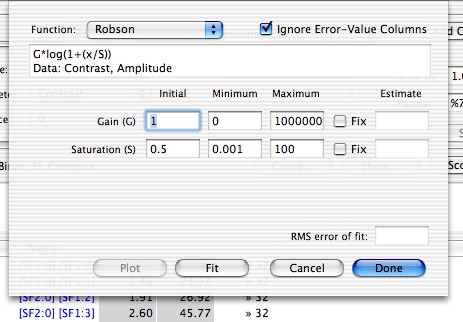
At the top sits a Function pop-up menu from which you can choose the function you want to fit. Underneath the chosen function Expo will display the function expression, with its parameters identified by uppercase letters. Below the expression appears a list of the required data columns. From left to right this specifies, in a comma-separated list, the types of data that must be contained in the selected columns in the analysis table, and the order in which they must appear.
If the number of columns selected in the table doesn't match the number required by the function chosen, Fit will be dimmed. (Expo counts selected columns per your setting of Ignore Error-Value Columns. If this is checked Expo ignores selected columns that contain error values.) The selected columns need not be contiguous, but for a sensible analysis each must contain data of the type specified in the list of requirements (when fitting a function Expo does not check that the data in a column are of the type required).
Below the function description Expo displays in rows, one for each parameter of the function, boxes in which you can enter the initial estimate of the parameter's value, and the maximum and minimum values between which STEPIT can range in finding a solution. The default values are reasonable for most purposes. Check Fix to lock the value of the parameter at the initial value.
To obtain an estimate of parameters, click Fit (this will be dimmed if the selected data in the table do not match the requirements of the function you have chosen). Expo will find and display an estimate.
Having obtained estimates of the parameters, you can plot the function on graphs of the selected data. To do this click Plot.
In fitting selected results, Expo never uses data from cells in table rows that are masked.
Clicking Done saves (internally) information about the type and fitting options of the function; this is retained for use in batch analysis.
You can open the main analysis window for any program that has data. In a running program the data are constantly being accumulated; you can configure Expo so that it will automatically update the analysis as new data are added.
To set up automatic analysis, choose Edit->Preferences…, and under the Windows tab check Update Windows Automatically. Expo revises the analysis for each row of the table as the scheduler completes a pass through the corresponding slot. Expo identifies the active slot/state by displaying its analyzed data in red. If you have a graph displaying selcted columns of data, Expo will update the graph regularly if you check Refresh Graphs Every N Seconds. Set N to control the frequency of updates.
If you have captured and saved the raw spike waveform, you can reanalyze it to generate a new set of spike times. You might want to do this if you originally ran the program with a poorly constructed spike template, or you want to recover the times of occurrence of a second spike. (If the raw spike waveform is available, the program’s status window will show how much was recorded).
Before reanalyzing the waveform, you should set up the template(s) you want to use. To do this, activate a window for the program that owns the data, then choose Data->Replay Spikes. This will play the raw waveform, just as it was originally recorded, and you can use the spike window to set thresholds and define templates. While replay is enabled, Expo displays in the upper right of the Spike Window the time (in minutes:seconds) from the start of recording. Expo cycles continuously through the stored waveform, resetting the time as it starts each cycle. To stop the replay choose Signals->Stop Replay.
| You cannot replay the raw spike waveform if any program is running or suspended. |
When you have set up your template(s) for the spikes being replayed, choose Data->Reanalyze Spikes to generate a new set of spike times. If the program that owns the data has an analysis window open, the cells are automatically updated to reflect the change. While Expo is replaying spikes you can reanalyze the times as often as you wish.