Revised:
Analysis routines fall into three groups: those for handling state events (values of parameters from routines), those for handling spikes, and those for handling continuously recorded analog signals. The analysis routines of each type become available when you choose the type of analysis from the tab in the main analysis window. If a program run has collected no spike data, the spike analysis routines are unavailable; if a program has collected no analog signals, the analog signal analysis routines are unavailable.
All analyses are undertaken on all passes through a state, unless the analysis scope has been restricted.
Mean, Variance, s.d., s.e.m., Sum, Count, Array », Times, Pass Indexes »
Count (µ), Count (s.d.), Count (s.e.m.), Count (array) », Count in Epochs », Times »», PST Histogram », PST Histogram (s.d.) », PST Histogram (var.) », PST Histogram (s.e.m.) », FT Amplitude (PSTH), FT Amplitude (µ), FT Amplitude (s.d.), FT Amplitude (s.e.m.), FT Amplitude (array) », FT Phase (PSTH), FT Phase (µ), FT Phase (s.d.), FT Phase (s.e.m.), FT Phase (array) », Amplitude Spectrum », Phase Spectrum », Interval Histogram », Minimum Intervals », Crosscorrelation », Crosscorrelation (s.e.m.) », Reverse Correlation »»
Array »», FT Amplitude (µ) »», FT Amplitude (s.d.) », FT Phase (µ) », FT Phase (s.d.) », Amplitude Spectrum »», Phase Spectrum »», Pass Mean »», Pass s.d. »», Pass s.e.m. »», Pass Variance »»
An analysis with a bullet before its name (•Count, •Times, •Pass Indexes) provides the same information regardless of which Routine and Parameter you have chosen for analysis.
Finds the mean of the recorded values of the chosen parameter.
Finds the variance of the recorded values of the chosen parameter. Variance values can be displayed as error bars on graphs.
Finds the standard deviation of the recorded values of the chosen parameter. s.d. values can be displayed as error bars on graphs.
Finds the standard error of the mean of the distribution of values of the chosen parameter. s.e.m. values can be displayed as error bars on graphs.
Finds the sum of the recorded values of the chosen parameter.
Puts recorded values of the chosen parameter in an array.
Counts the number of times the value of the chosen parameter was recorded (subject to any scope restrictions).
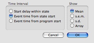
Provides various analyses of the times at which routine events were recorded. When you click Set to install this analysis in selected cells, Expo displays the following sheet:
You specify one of three time intervals to be measured: the delay between the start of a slot and the state becoming active (useful if you want to know about random start delays); the interval between the state becoming active and the recording event; the interval between the start of the program and the recording event. s.e.m. or s.d. values can be displayed as error bars on graphs.
| Expo records event times to the nearest 100µsec. Nevertheless, the times at which state events are actually recorded are generally quantized on a larger scale. When you use a button click or a keypress to trigger the recording of events, Expo will register the triggering event on the next timebase tick. If your timebase is derived from a monitor, this could be as much as 13 msec after the triggering event. The Read Key routine copes with this problem by saving in its event record the exact time at which the key was pressed. |
Builds an array of the absolute positions occupied by this cell’s slot/substate in the sequence of all passes through all states during an experimental run. The settings of Routine, Parameter and Instance are ignored.
All spike analysis routines act on spikes accumulated during each pass through a state. The default interval during which spikes are accumulated runs from activation of the state (i.e., when it is triggered) until it is stopped. This default interval can be modified by changing the span of analysis via the spike analysis tab.
Counts the average count of spikes recorded when the state was active.
Finds the standard deviation of the number of spikes recorded when the state was active. Count (s.d.) values can be displayed as error bars on graphs.
Finds the standard error of the mean number of spikes recorded when the state was active. Count (s.e.m.) values can be displayed as error bars on graphs.
Forms an array of counts of spikes recorded when the state was active. The array contains every occurrence permitted by Scope.
Forms an array of average counts of spikes recorded in successive epochs when the state was active. When you click Set to install this analysis in selected cells, Expo displays a sheet through which you can specify the duration of the Epochs over which spikes will be counted.
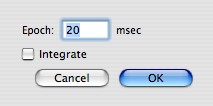
Counts from successive epochs are integrated if you check Integrate.
Forms a two-dimensional array in which the outer dimension indexes passes (sweeps) and the inner dimension indexes the time of occurrence of each spike within a pass. When you click Set to install this analysis in selected cells, Expo displays a sheet through which you specify the particulars of the analysis.
The arrays can be aligned to a time marker provided by a routine that was active during the state. (Currently the routines Pulse and Analog Bounds provide markers.) To align the averaging to a marker, choose the routine from the Alignment popup menu, and specify the instance (these items are dimmed if no routines called in the state generate markers). The default alignment does nothing. Any alignment offset is applied in addition to any adjustment of the analysis span defined by the span setting in the spike analysis tab.
Array locations for which there is no corresponding spike time have a value of 0.
When displaying spike time arrays in graphs, EXPO can show them as it would any other two-dimensional arrays, or can display them in a raster plot. To enable the raster display choose Data->Graph Options… and check Display as Raster when Possible.
Forms an array of bins of specified width, and places in each bin the average number of spikes collected during its interval. When you click Set to install this analysis in selected cells, Expo displays a sheet through which you specify the particulars of the analysis.
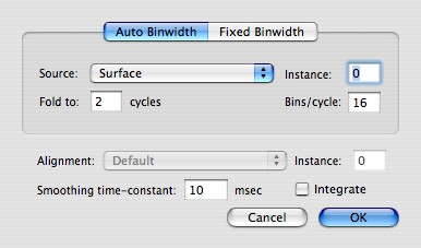
Expo can derive the binwidth automatically from any routine used in a state, if that routine generates a frequency signal (e.g., flicker, grating drift rate). To use a frequency source, click the Auto Binwidth tab, and choose the frequency source you want (you cannot choose the tab if no frequency source has been used). If the frequency source is within a routine that was used more than once in the state, you must also specify the Instance. Instances are numbered from 0. You must also specify through Fold to the number of cycles of the frequency source to be represented in the array of bins (the default is 2; enter 0 if you don't want any folding). You should specify through Bins/cycle the number of bins per cycle (the default is 16). To use a fixed binwidth, click the Fixed Binwidth Tab, and enter the binwidth you require (the default is 20 msec). If you want the histogram folded to a fixed number of bins, specify that number (0 for no folding).
The histogram passes can be aligned to a time marker provided by a routine that was active during the state. (Currently the routines Pulse and Analog Bounds provide markers.) To align the averaging to a marker, choose the routine from the Alignment popup menu, and specify the instance (these items are dimmed if no routines called in the state generate markers). The default alignment does nothing. Any alignment offset is applied in addition to any adjustment of the analysis span defined by the span setting in the spike analysis tab.
To apply a smoothing time-constant to the count in each bin, enter the value at Smoothing time-constant. A value of 0 turns off smoothing. The default is 10msec.
To obtain an integrated histogram (each bin adds in the count of the preceding bin) check Integrate.
Forms an array of bins of specified width, and places in each bin the standard deviation of the number of spikes collected during its interval. Settings are the same as for PST Histogram above. PST Histogram (s.d.) values can be displayed as error bars on graphs.
Forms an array of bins of specified width, and places in each bin the variance of the number of spikes collected during its interval. Settings are the same as for PST Histogram above. PST Histogram (var.) values can be displayed as error bars on graphs.
Forms an array of bins of specified width, and places in each bin the standard error of the number of spikes collected during its interval. Settings are the same as for PST Histogram above. PST Histogram (s.e.m.) values can be displayed as error bars on graphs.
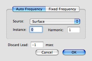
Finds the amplitude of the specified frequency component in the spike train collected while the state was active. Expo averages the spike trains collected during every pass through the state then takes the Fourier transform of it. For a different analysis see FT Amplitude (µ), below. When you click Set to install this analysis in selected cells, Expo displays a sheet through which you specify the particulars of the analysis.
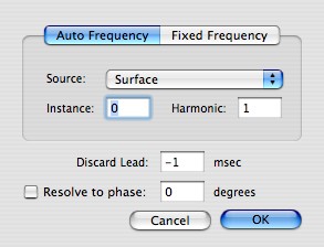
You can specify the frequency directly by clicking Fixed Frequency and entering the appropriate frequency in the box; if the frequency is generated by a routine in a state, click Auto Frequency and choose the source routine from the pop-up menu. If the source is from a routine that was used more than once in the state, you must also specify the Instance. Instances are numbered from 0. You must then specify the harmonic you want analyzed. You can exclude the initial segment of the spike train from the analysis. To specify this enter the segment duration at Discard Lead. Expo will automatically choose an amount to discard (never less than .125 sec) if you enter –1. You can force the amplitude to be resolved to a particular phase. To do this check Resolve to Phase and enter the phase (in degrees) to which you want the amplitude resolved.
| When you specify a frequency of 0 (to recover the mean spike rate), Expo will deliver a result only if Discard Lead is set to 0. |
Finds the mean amplitude of the specified frequency component in the set of spike trains collected while the state was active. Expo computes the transform separately for the spikes collected during each pass through the state, then averages the resulting amplitudes. For a different analysis see FT Amplitude (PSTH), above. Setup details as for FT Amplitude (PSTH).
Finds the standard deviation of the amplitude of the specified frequency component in the set of spike trains collected while the state was active. Other details as for FT Amplitude (µ), above. FT Amplitude (s.d.) values can be displayed as error bars on graphs.
Finds the standard error of the amplitude of the specified frequency component in the set of spike trains collected while the state was active. Other details as for FT Amplitude (µ), above. FT Amplitude (s.e.m.) values can be displayed as error bars on graphs.
Finds the amplitude of the specified frequency component in the spike train collected while the state was active. Expo computes the transform separately for the spikes collected during each pass through the state, then creates an array of the resulting amplitudes. Setup details as for FT Amplitude (PSTH).
Finds the phase of the specified frequency component in the spike train collected while the state was active. Expo averages the spike trains collected during every pass through the state then takes the Fourier transform of it. For a different analysis see FT Phase (µ). When you click Set to install this analysis in selected cells, Expo displays a sheet through which you specify the particulars of the analysis.
You can specify the frequency directly by clicking Fixed Frequency and entering the appropriate frequency in the box; if the frequency is generated by a routine in a state, click Auto Frequency and choose the source routine from the pop-up menu. If the source is from a routine that was used more than once in the state, you must also specify the Instance. Instances are numbered from 0. You must then specify the harmonic you want analyzed. You can exclude the initial segment of the spike train from the analysis. To specify this enter the segment duration at Discard Lead. Expo will automatically choose an amount to discard (never less than .125 sec) if you enter –1.
Finds the mean phase of the specified frequency component in the set of spike trains collected while the state was active. Expo computes the transform separately for the spikes collected during each pass through the state, then averages the resulting phases. For a different analysis see FT Phase (PSTH) (above). Setup details as for FT Phase (PSTH), above.
Finds the standard deviation of the phase of the specified frequency component in the set of spike trains collected while the state was active. Other details as for FT Phase (µ), above. FT Phase (s.d.) values can be displayed as error bars on graphs.
Finds the standard error of the phase of the specified frequency component in the set of spike trains collected while the state was active. Other details as for FT Phase (µ), above. FT Phase (s.e.m.) values can be displayed as error bars on graphs.
Finds the phase of the specified frequency component in the spike train collected while the state was active. Expo computes the transform separately for the spikes collected during each pass through the state, then creates an array of the resulting phases. Setup details as for FT Phase (PSTH).
Uses a Fast Fourier Transform (FFT) to find the amplitudes of the fundamental frequency and its first 31 harmonics in the set of spike trains collected while the state was active. Expo computes the transform from the average of the spikes collected during each pass through the state, and puts them in an array. The first element in the array is the amplitude of F0, the second F1, etc.
When you click Set to install this analysis in selected cells, Expo displays a sheet through which you specify the fundamental frequency. See the description of FT Phase (PSTH).
As for Amplitude Spectrum » (above) except that it finds the phases of the fundamental frequency and its first 31 harmonics.
Calculates the intervals between successive spikes and produces a distribution of them in an array of bins of specified width. Expo sets the array size to 250 bins, and the last bin contains all intervals appropriate to it or longer.
When you click Set to install this analysis in selected cells, Expo displays a sheet through which you specify the width of the bins into which intervals will be placed. The default bin width is 30 msec.
Forms an array (of length equal to the number of times the state/slot was run) of the shortest interspike interval found during each pass.
Computes a cross-correlation between two spike trains. When you click Set to install this analysis in selected cells, Expo displays a sheet through which you specify the second of the two spike identifiers (the first is whatever Spike you have specified in the Spike tab of the main window).
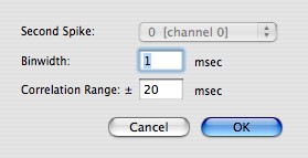
If both spikes have the same identifier, the routine performs an autocorrelation (if only one spike was recorded, the menu is dimmed). Binwidth specifies the width of the bins in which spikes are accumulated for the analysis, and Correlation Range specifies the range of time separations (around 0) over which the correlation is computed. The result is normalized such that the autocorrelation has a maximum value of 1.
Computes the standard error of the cross-correlation between two spike trains. Other details as for Crosscorrelation » (above). Values can be displayed as error bars on graphs
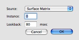
Computes a reverse correlation on the spike train to recover the average stimulus at a specified time before each spike. Source routine specifies the display routine that controlled the generation of stimuli (currently only the Surface Matrix routine can do this). Instance specifies the instance of the routine. Expo uses Source and Instance to recover from the event queue the information needed to reconstruct the average two dimensional array of stimulus elements at the Lookback interval before each spike.
The result is a N x N array in which each element is the average value of the varying attribute of the corresponding element in the Surface Matrix. The outer dimension of the array represents matrix columns and the inner dimension matrix rows, with values increasing from bottom to top, and left to right. Expo knows the stimulus attribute that is varying, and delivers values in the natural unit for that attribute, as follows:
| Reverse Correlation is enabled in the menu of analysis options only if the data were collected by a program that used the Surface Matrix routine to display stimuli. |
When displaying reverse correlation results in graphs, EXPO can show them as it would any other two-dimensional arrays, or can display them in a two-dimensional matrix plot in which the grayscale value of each point represents the value of the relevant parameter in the stimulus array. To enable the matrix display choose Data->Graph Options… and check Display as Matrix when Possible.
All analog analysis routines act on signals accumulated during each pass through a state. The default window during which signals are accumulated runs from activation of the state (i.e., when it is triggered) until it is stopped. This default window can be modified by changing the span of analysis via the analog analysis tab.
Forms a two-dimensional array of the analog signals sampled when the state was active, computed over all occurrences permitted by Scope. The first (outer) dimension indexes the channel, and the second (inner) dimension indexes the sample.
Finds the amplitude of the specified frequency component in the analog signal collected while the state was active. The result is the average of the amplitudes found by undertaking a Fourier transform separately on each pass.
When you click Set to install this analysis in selected cells, Expo displays a sheet through which you specify the particulars of the analysis. You can specify the frequency directly by clicking Fixed frequency and entering the appropriate frequency in the box; if the frequency is one generated by a routine in a state (e.g., flicker, grating drift rate), you can choose the frequency source by clicking Auto frequency and choosing the source routine from the pop-up menu. If the frequency source is within a routine that was used more than once in the state, you must also specify the Instance. Instances are numbered from 0. You must then specify the harmonic you want analyzed.
As FT Amplitude (mean), except that standard deviation is computed. FT Amplitude (s.d.) values can be displayed as error bars on graphs.
As FT Amplitude (mean), except that the average phase is computed.
As FT Phase (mean), except that the standard deviation is computed. FT Phase (s.d.) values can be displayed as error bars on graphs.
Uses a Fast Fourier Transform (FFT) to find the amplitudes of the fundamental frequency and up to 8191 harmonics in the set of analog signals collected while the state was active. Expo computes the transform on the average of the samples collected during each pass through the state, and puts the results in an array that is as long as is needed to contain them. The result is a two-dimensional array, with the first dimension indexing the channel, and the second dimension indexing the harmonic (the first element is the amplitude of F0, the second F1, etc.). Since the fundamental sampling rate for analog signals is limited by the analog sampling hardware, Expo will show only the harmonics that can be calculated for the sampling rate used. Expo uses a vector-optimized FFT when possible.
When you click Set to install this analysis in selected cells, Expo displays a sheet through which you must specify the fundamental frequency. You can fix this by entering the appropriate frequency in Fixed frequency; if you enter 0, Expo automatically sets the period of the fundamental frequency to be the duration of the sweep. If the frequency is one generated by a routine in a state, you can get the frequency source by clicking Auto frequency and choosing the source routine from the pop-up menu.
As Amplitude Spectrum »», except that the phase spectrum is computed.
Finds, for each channel being scanned, the mean value of the analog signals sampled on each pass through the state. The result is a two dimensional array, with the first dimension indexing the channel, and the second dimension indexing the pass through the state.
As Pass Mean »», except that the standard deviation is computed. Pass s.d. »» values can be displayed as error bars on graphs.
As Pass Mean »», except that the standard error of the mean is computed. Pass s.e.m. »» values can be displayed as error bars on graphs.
As Pass Mean »», except that the variance is computed. Pass Variance »» values can be displayed as error bars on graphs.
Forms a two-dimensional array of the analog signals sampled on the First Channel (the setting of Second Channel is ignored), computed over all occurrences permitted by Scope. The first (outer) dimension indexes the pass, and the second (inner) dimension indexes the sample.