Revised:
Expo provides two ways to export data for analysis by Matlab or other programs.
The first exports the Analysis table as an Excel spreadsheet. For this format Expo does most of the unpacking and structuring, and often much of the analysis, but you can work only with the data elements in the ways that Expo exposes through its Analysis window. Jonathan Peirce has written a collection Matlab scripts to work with Expo data exported in spreadsheet form.
The second export format provides a complete representation of a data set as an XML document. This structures the data in a way that allows you to do anything you want with them, but does none of the unpacking and linking of different kinds of data that are done by Expo's analysis functions. Julian Brown has written a suite of Matlab routines to handle this. These routines read, organize and analyze the data elements contained in XML documents.
Both collections of Matlab routines are included with the Expo distribution. The following sections describe how to use them.
The following account from Neel Dhruv (ndhruv@cns.nyu.edu) describes how to use Jonathan Peirce's Matlab routines to import spreadsheet-formatted data.
This section assumes you are generally familiar with data analysis in Expo. To produce spreadsheets as tab-delimited .xls spreadsheets for Microsoft Excel, use the batch analysis capabilities. The files Expo produces are readable directly by Matlab, but for the Matlab import filters to be maximally useful the Expo analysis that gives rise to the data should follow certain naming and formatting conventions.
| The Excel (.xls) files Expo produces contain plain text. If you open a file in Excel it will convert the data to its private (binary) format, and when you close the file will ask if you want to save changes. If you do save changes, Matlab will be unable to read the file subsequently. |
Here is a summary of the steps in organizing the Analysis. For a fuller treatment see the discussion of batch analysis
Open a model data file, then open an Analysis window and create or apply a template for the analysis you want to undertake. If you want to use a single template for lots of data sets collected by a variety of Expo programs, build it for the data set that contains the largest number of rows (Expo can be set to analyze a data set using a template the contains too many rows, but it will never analyze a data set with a template that contains too few rows).
Highlight the columns of data that you want to export. If you have masked a row, no data from that that row will be exported. Column names appear as field names in the .mat files produced by the import filtering. Name your template columns carefully. A column name must contain no space. The import will also handle specially data from any column named ‘xpos’ (see below).
Choose Data->Analyze Batch to start the batch analysis. In the panel Expo displays choose File: Table Data and click OK.
A panel will appear asking you to pick the location and filename of the output file to be created. You can choose to output the complete analysis (from all data files) in one file or in a separate file for each experiment; in the latter case each file will be given the base name you specify and a qualifier that distinguishes it, taken from the name of the Expo datafile.
A second panel will appear asking you to choose the files containing data to be analyzed. Select those you care about. If you want further filtering by the program that collected the data, specify that. (Leave the program name empty if you want to analyze data in all the chosen files.) Click OK to undertake the analysis.
This section assumes you are generally familiar with Matlab, and that the collection of relevant M files (in the distribution folder "ExpoXLSToMatlab") is available somewhere on your path. The M files exploit naming conventions used in the Lennie lab, but can be adapted easily to use others.
With Matlab running under X11, type ‘expoximport’ or ‘expoximport(1)’ at the command prompt. This will bring up a series of X11 dialog boxes to lead you through the steps. Using expoeximport(1) will give you feedback about each set of experimental data imported.
In the dialog box, navigate to the folder containing the .xls files that you want to import.
After you click OK, a new dialog box appears that will prompt you to enter a search string that names source files you wish to import. Note that this uses wildcards (*).
Next, select the output file location and enter the name you want to assign to the Matlab .mat file that will contain the data. If you select an existing .mat file as the output file, new data will be appended appropriately.
The organization of data in the .mat file exploits a naming convention that Expo uses by default when saving data files. This convention splits a data file name into three parts, an aribitrary root name (for example, an animal/cell identifier), followed by #, then a numerical suffix (a particular experimental run on the cell), followed in square brackets by the name of the Expo program that collected the data. expoximport organizes imported data first by the base name, then under that root name by program name and suffix.
The .mat file produced contains a nested structure tree. At the top level, there is a structure for each root name. This structure is named for the root, and a new top level entry is created automatically when a new root name is encountered.
|
When naming a structure at the top level, expoximport currently adds an ‘m’ to the beginning of each root name that doesn’t already begin with 'm'. |
Each top level entry contains an array of structures, one for each experiment run under that root name. Second level structures in this array are named with the program name followed by an underscore followed by the suffix. Thus data for multiple experiments run on the same cell (which will have the same root name) will appear as different second-level entries under the same root structure.
Data imported with a root name for which entries already exist in the .mat file will be appended, indexed under the appropriate suffix and program name. (If the index is already used, the new data will replace the old.)
In forming the names of second-level entries, expoximport currently strips leading ‘get_’ and ‘twin_’ from the program name. For example:
Expo datafile 184a#0[get_or8] --> Batch Analysis --> 184.xls --> expoximport --> m184a.or8_0
Each second level entry contains fields that are the column data from the Expo analysis that gave rise to it.
If you used ‘xpos’ as the title of a column to be exported, expoximport interprets the contents of the column as an indicator that allows it to separate data for left and right eyes. Negative values represent left eye, positive values, right eye. This may be useful if a cell is binocular, and you ran two experiments with nearly identical stimuli. In such a case, a new level of the tree is inserted between the root layer and the program layer, with the substructures ‘l’ or ‘r’. For example:
Expo datafile 184a#0[get_or8] (which has a selected column titled 'xpos')--> Batch Analysis --> 184.xls(which has a column in the sheet titled 'xpos') --> expoximport --> m184a.l.or8_0 in which the field names are the columns selected for Batch Analysis in Expo.
The following account from Jim Müller (jim.muller@stanford.edu) and Julian Brown (julian@monkeybiz.stanford.edu) describes how to use Julian's suite of Matlab routines to import and analyze XML-formatted data. These routines require Matlab 7 (release 14).
|
Changes to the Matlab routines since first release: 30 March 2005. Added parsing code for the matrix and the GetPasses argument matrixElement. Now parses a complete description of the program's slots (XML export version 1.1). 08 March 2005. Added a new function GetVariable that enables you to extract a parameter value from a program. 13 Jan 2005. Added GetTransitionProbabilities 05 Jan 2005. Several bug fixes, most importantly two in ReadExpoXML. Very large files with more than 32,767 passes are now processed correctly. Files generated by programs that have no Comment are now processed correctly. This release also adds routines GetSpikeCounts and MergeExpoDataSets, described below. |
The following discussion assumes you are generally familiar with the organization of an Expo program, and the major elements of an Expo dataset. These are exposed as text objects in the XML file and can be inspected with any editor. Appendix B describes the internal organization of an Expo program (reflected in the XML export), and Appendix C describes the organization of data elements, some of which are reflected in the XML export.
The Expo distribution includes a suite of Matlab routines in the folder named "ExpoXMLToMatlab." To use these routines you will need to add the folder and the sub-folder "ExpoXMLToMatlab/Helper functions" to your Matlab path.
To import an XML file into Matlab, use the routine
ReadExpoXML(filename, [doSpikeWaveforms]).
The optional doSpikeWaveforms parameter determines whether to include any raw spike waveform in the import. If there is no raw spike waveform in the XML file this switch is ignored.
ReadExpoXML may take a few minutes-on a G5 perhaps 2 minutes per hour of data collected (if the raw spike waveform is processed, it takes about one hour per hour of data collected.) The function reports at various times on how much of the data set it has processed. Once finished, ReadExpoXML saves the imported data as a Matlab .mat file which can be reloaded quickly later. The .mat file takes the name filename but with the .xml extension replaced by .mat. The .mat file is typically less than half the size of the original XML file.
If your invocation of ReadExpoXML looks like this:
z = ReadExpoXML('192h#3[get_or_var].xml', 1)
the function will leave in working memory a Matlab structure z (referred to in the Matlab code as expoDataSet). The expoDataSet object can be reinstated at a later time from the .mat file by the following command:
z = load('expofile.mat');
It contains the fields blocks, slots, passes, spiketimes, waveforms, analog, environment, each of which contains further sub-structures that you can easily browse in the Matlab environment. By doing so you can find information about the program from blocks and slots and about other Expo settings in environment. The data are described by passes, spiketimes, waveforms and analog, but are always more easily accessed using the following routines:
Most of the remaining functions require you to supply a vector of pass IDs such as is returned by GetPasses. Note that for these routines, as in Expo, all IDs are 0-based, unlike Matlab array indices, which are 1-based.
As an example, let’s analyze data from a simple delayed, memory-guided saccade program:
z = load('w041220c#4[Delayed MG Saccades].mat');
or
z = ReadExpoXML('w041220c#4[Delayed MG Saccades].xml’);
While we recorded presaccadic responses from his superior colliculus, a monkey was asked to fixate (a slot containing the block ‘FP’), view a briefly-presented target (‘FP+Targ’), wait (another slot containing ‘FP’), then was cued (‘Presac’) to make a saccade. A few additional blocks assured that the monkey completed the saccade, and rewarded him for it, ending with block ‘Valid’. Our analysis will make use of three of these slots, and because slots don’t always have names, we will get them using the names of the blocks they contain. Each of these blocks happens to define a single slot.
vstimslot = GetSlots(z, 'FP+Targ');
presacslot = GetSlots(z, 'Presac');
validslot = GetSlots(z, 'Valid');
We want to analyze exactly those trials which are valid, and GetPasses provides an easy way to do this: we always supply the slot argument as validslot, but we indicate which slot we really want using an offset. This is just as one would do with the Current button in the Expo Analysis window. Because all valid trials pass through each of these slots in turn, simple subtraction is enough to compute offset:
vstim = GetPasses(z, validslot, vstimslot - validslot);
presac = GetPasses(z, validslot, presacslot - validslot);
vstim and presac have the same length, and each represents the list of all valid trials. Each is a list of passIDs, and passIDs are the key to accessing information about what that particular block (e.g. ‘Presac’) did on an individual trial.
In this experiment saccade targets at different locations were interleaved. Let’s restrict analysis to just one ‘preferred’ target, the leftmost one. We use GetEvents to get the target positions. It functions much like Expo Analysis Events.
x = GetEvents(z, vstim, 'Surface', 'Target', 0, 'X-position', 'deg');
You will recognize most of its arguments as the exact names of Expo routines, labels, and parameters. We now filter our lists of passes and keep only those from trials featuring the ‘preferred’ target, using standard Matlab operations.
xunique = sort(unique(x));
vstim_preferred = vstim(x == xunique(1));
presac_preferred = presac(x == xunique(1));
Now we can examine the eye traces for valid saccades to this preferred target. ‘Presac’ was written to use the Expo routine Analog Bounds to monitor eye position, and its Time parameter gives the time at which the saccade began. We retrieve these times in msec following the start of the ‘Presac’ state.
sacbegin = GetEvents(z, presac_preferred, 'Analog Bounds', '', 0, 'Time', 'msec');
To retrieve the eye-traces from a ±100 msec interval centered at this time we simply call GetAnalog, which works much like Expo Analysis Analog. We ask that the traces be returned in degrees and tell it that we are supplying time bounds in msec. It obligingly returns the sampleInterval in the same units, msec.
[eyex firstSampleTimes sampleInterval]
= GetAnalog(z, 0, presac_preferred, sacbegin-100, 200, 1, 'msec','deg');
eyey = GetAnalog(z, 1, presac_preferred, sacbegin-100, 200, 1, 'msec','deg');
We use standard Matlab commands to plot them:
eyet = -100:sampleInterval:100;
figure; plot(eyet, eyex, 'LineWidth',2);
figure; plot(eyet, eyey, 'LineWidth',2);
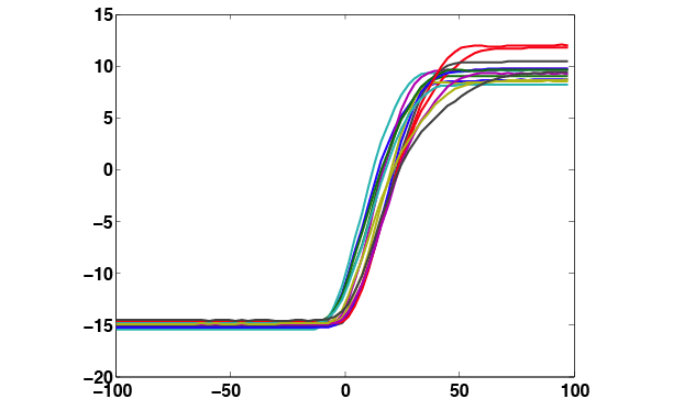
The plot of x-values would look something like this:

In general, we might want to plot analog traces, which are sampled with one accurate (100 µsec) clock, so that they are aligned to state transition boundaries, which are generated by a different accurate clock. For low analog sampling rates, this means that in plots such as the one above, each trace has a firstSampleTime that varies from the next by as much as several msec. To get this detail right one can use the following Matlab incantation to shift each trace by its firstSampleTime:
plot(eyet' * ones(size(firstSampleTimes)) + ones(size(eyet')) * firstSampleTimes, eyex');
Corresponding spikes can be gotten by a call to GetSpikeTimes, which works much like Expo Analysis Spike Times.
spikes = GetSpikeTimes(z, 0, presac_preferred, sacbegin-1000, 1500, 1, 'msec');
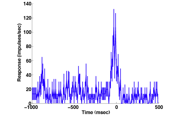
These spike times are from intervals beginning 1000 msec before each saccade and lasting 1500 msec. Note that the times are relative to the beginning of that interval, so the earliest spikes returned for each trial have values near zero. To create a a post-stimulus time histogram we call GetPSTH, which interprets its time arguments (and expresses its result t) in this same way, and plot what it returns.
[m, sem, t] = GetPSTH(spikes, 0, 10, 1500,'msec','impulses/sec');
PlotPSTH(m, sem, t-1000,'msec','impulses/sec');
For plotting purposes we subtracted 1000 msec from all the times, just as we subtracted 1000 msec from sacbegin when we specified the time intervals in the first place. Thus the x-axis is labeled relative to the beginning of the saccade.
