Contents

%Lab 8 This lab introduces resampling methods
%Bootstrapping, Monte Carlo, several use cases

%Init
clear all
close all
clc

%Seed the random number generator
s = RandStream('mt19937ar','Seed',sum(round(clock)));
RandStream.setGlobalStream(s);

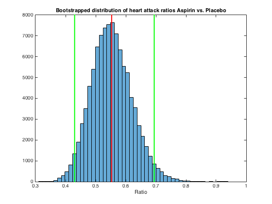
1 Classic Efron - does Aspirin prevent heart attacks

nA = 11037; %Aspirin takers
nHA = 104; %Aspirin takers with heart attacks
nP = 11034; %Placebo takers
nHP = 189; %Of those, #heart attacks
nSamples = 1e5; %Number of times to resample (large-ish)
ratio = zeros(nSamples,1); %Initialize, preallocate

A1 = ones(nHA,1); %This represents aspirin takers who had heart attacks
A2 = zeros(nA-nHA,1);%This represents aspirin takers who did not
P1 = ones(nHP,1); %Same for placebo
P2 = zeros(nP-nHP,1); %Same thing

%Make the data vectors
A = [A1;A2]; %Stack all people who took aspirin, regardless of outcome
P = [P1;P2]; %Stack all the placebo takers


%NOW: To calculate the distribution of sample means, resample from the
%sample. In English: Sample with replacement.

for ii = 1:nSamples %Do this nSamples times. This is for didactic clarity. You could do this without a loop by drawing 1000 columns at once.
indicesA = randi(nA,[nA 1]); %Draw random integers. Largest: Sample size, sample size times
indicesP = randi(nP,[nP 1]); %Draw random integers. Largest: Sample size, sample size times
ratio(ii) = sum(A(indicesA))/sum(P(indicesP)); %This is the ratio of HA in virtual sample
end

%Now that we bootstrapped a distribution of ratios, we calculate the CI
%First: We need to sort the values
sortedRatio = sort(ratio); %Sort it
lowerBoundIndex = round(nSamples/100*2.5); %Find the index of the lower bound
upperBoundIndex = round(nSamples/100*97.5); %Apologies for hardcoding. Exercise for user: Make this a variable, i.e. to get the 50% CI
lowerBound = sortedRatio(lowerBoundIndex); %Find actual lower bound value
upperBound = sortedRatio(upperBoundIndex); %Find actual higher bound value

%Plot histogram
figure
histogram(ratio,50); %50 bins
xlabel('Ratio')
%Add lines representing mean and CI of this distribution
line([mean(ratio) mean(ratio)], [min(ylim) max(ylim)],'color','r','linewidth',2)
line([lowerBound lowerBound], [min(ylim) max(ylim)],'color','g','linewidth',2)
line([upperBound upperBound], [min(ylim) max(ylim)],'color','g','linewidth',2)
title('Bootstrapped distribution of heart attack ratios Aspirin vs. Placebo')

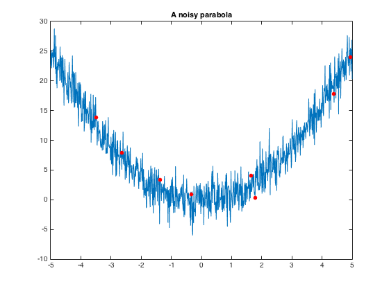
2 Using resampling methods for cross-validation

%1 Get our samples
%2 Fit polynomials
%3 Leave one out and resample

numPoints = 8; %Eero's choice
noiseMagnitude = 2; %This dial will allow you to tune up and down the effect of noise
x = -5:0.01:5; %Let's get 1001 equally spaced points between -5 and 5
y = x.^2 + noiseMagnitude .* randn(1,length(x)); %Parabola, with some additive random noise

figure
plot(x,y)
title('A noisy parabola')

%1 Find the 8 points on this parabola
samplingIndices = randi(length(x),[numPoints,1 ]) ;%Find 8 random indices in the larger vector
hold on;
plot(x(samplingIndices),y(samplingIndices),'.','color','r','markersize',20)

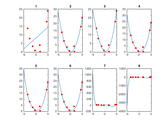
% 2 (Over)fitting polynomials and calculating RMSE
RMSE = []; %Our figure of merit
figure
for ii = 1:numPoints
    subplot(2,4,ii)
    p = polyfit(x(samplingIndices),y(samplingIndices),ii); %Use randomly drawn data points and fit it with polynomials of degree ii
    %p will be a vector of weights/coefficients of the polynomial
    yHat = polyval(p,x); %Evaluate these estimated p's at all values of x
    plot(x,yHat)
    hold on
    plot(x(samplingIndices),y(samplingIndices),'.','color','r','markersize',20)
    title(num2str(ii))
    RMSE(ii) = sqrt(mean((y(samplingIndices)-yHat(samplingIndices)).^2));
end

figure
plot(1:numPoints,RMSE)
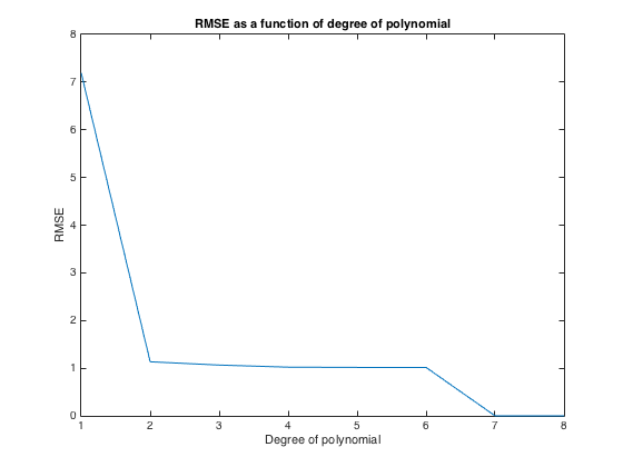
title('RMSE as a function of degree of polynomial')
xlabel('Degree of polynomial')
ylabel('RMSE')

%As you can see, the RMSE keeps dropping as we add terms to the polynomial.
%But we are fitting to noise. Because the underlying data was noisy.
%Fitting to noise: Overfitting.

%So how do we pick a model here?

%Resampling methods, leaving one out to cross-validate the appropriate
%number of terms in the model

numSamples = 1e2; %New number of samples
RMSE = zeros(numSamples,numPoints-1); %Reinitialize RMSE

for ii = 1:numSamples %Do this as many times as we want to bootstrap it
testIndex = randi(numPoints,1); %This is the index of the point we want to predict
testSet = samplingIndices(testIndex); %Get the index of the sampling points that will form our test set
trainingSet = samplingIndices; %Make a copy of the sampling indices
trainingSet(testIndex,:) = []; %Remove the indices of the set set. As we leave only one out, we will just delete one

    for jj = 1:numPoints-1
    p = polyfit(x(trainingSet),y(trainingSet),jj); %We now fit to the training set, not the full set
    yHat = polyval(p,x); %Evaluate these estimated p's at all values of x
    RMSE(ii,jj) = sqrt((y(testSet)-yHat(testSet)).^2);
    end
end

%Logic: FIT to the training set, but calculate your ERROR with the test set

figure
plot(1:numPoints-1,mean(RMSE))
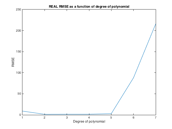
title('REAL RMSE as a function of degree of polynomial')
xlabel('Degree of polynomial')
ylabel('RMSE')

Warning: Polynomial is not unique; degree >= number of data points. 
Warning: Polynomial is not unique; degree >= number of data points. 
Warning: Polynomial is not unique; degree >= number of data points. 
Warning: Polynomial is not unique; degree >= number of data points. 
Warning: Polynomial is not unique; degree >= number of data points. 
Warning: Polynomial is not unique; degree >= number of data points. 
Warning: Polynomial is not unique; degree >= number of data points. 
Warning: Polynomial is not unique; degree >= number of data points. 
Warning: Polynomial is not unique; degree >= number of data points. 
Warning: Polynomial is not unique; degree >= number of data points. 
Warning: Polynomial is not unique; degree >= number of data points. 
Warning: Polynomial is not unique; degree >= number of data points. 
Warning: Polynomial is not unique; degree >= number of data points. 
Warning: Polynomial is not unique; degree >= number of data points. 
Warning: Polynomial is not unique; degree >= number of data points. 
Warning: Polynomial is not unique; degree >= number of data points. 
Warning: Polynomial is not unique; degree >= number of data points. 
Warning: Polynomial is not unique; degree >= number of data points. 
Warning: Polynomial is not unique; degree >= number of data points. 
Warning: Polynomial is not unique; degree >= number of data points. 
Warning: Polynomial is not unique; degree >= number of data points. 
Warning: Polynomial is not unique; degree >= number of data points. 
Warning: Polynomial is not unique; degree >= number of data points. 
Warning: Polynomial is not unique; degree >= number of data points. 
Warning: Polynomial is not unique; degree >= number of data points. 
Warning: Polynomial is not unique; degree >= number of data points. 
Warning: Polynomial is not unique; degree >= number of data points. 
Warning: Polynomial is not unique; degree >= number of data points. 
Warning: Polynomial is not unique; degree >= number of data points. 
Warning: Polynomial is not unique; degree >= number of data points. 
Warning: Polynomial is not unique; degree >= number of data points. 
Warning: Polynomial is not unique; degree >= number of data points. 
Warning: Polynomial is not unique; degree >= number of data points. 
Warning: Polynomial is not unique; degree >= number of data points. 
Warning: Polynomial is not unique; degree >= number of data points. 
Warning: Polynomial is not unique; degree >= number of data points. 
Warning: Polynomial is not unique; degree >= number of data points. 
Warning: Polynomial is not unique; degree >= number of data points. 
Warning: Polynomial is not unique; degree >= number of data points. 
Warning: Polynomial is not unique; degree >= number of data points. 
Warning: Polynomial is not unique; degree >= number of data points. 
Warning: Polynomial is not unique; degree >= number of data points. 
Warning: Polynomial is not unique; degree >= number of data points. 
Warning: Polynomial is not unique; degree >= number of data points. 
Warning: Polynomial is not unique; degree >= number of data points. 
Warning: Polynomial is not unique; degree >= number of data points. 
Warning: Polynomial is not unique; degree >= number of data points. 
Warning: Polynomial is not unique; degree >= number of data points. 
Warning: Polynomial is not unique; degree >= number of data points. 
Warning: Polynomial is not unique; degree >= number of data points. 
Warning: Polynomial is not unique; degree >= number of data points. 
Warning: Polynomial is not unique; degree >= number of data points. 
Warning: Polynomial is not unique; degree >= number of data points. 
Warning: Polynomial is not unique; degree >= number of data points. 
Warning: Polynomial is not unique; degree >= number of data points. 
Warning: Polynomial is not unique; degree >= number of data points. 
Warning: Polynomial is not unique; degree >= number of data points. 
Warning: Polynomial is not unique; degree >= number of data points. 
Warning: Polynomial is not unique; degree >= number of data points. 
Warning: Polynomial is not unique; degree >= number of data points. 
Warning: Polynomial is not unique; degree >= number of data points. 
Warning: Polynomial is not unique; degree >= number of data points. 
Warning: Polynomial is not unique; degree >= number of data points. 
Warning: Polynomial is not unique; degree >= number of data points. 
Warning: Polynomial is not unique; degree >= number of data points. 
Warning: Polynomial is not unique; degree >= number of data points. 
Warning: Polynomial is not unique; degree >= number of data points. 
Warning: Polynomial is not unique; degree >= number of data points. 
Warning: Polynomial is not unique; degree >= number of data points. 
Warning: Polynomial is not unique; degree >= number of data points. 
Warning: Polynomial is not unique; degree >= number of data points. 
Warning: Polynomial is not unique; degree >= number of data points. 
Warning: Polynomial is not unique; degree >= number of data points. 
Warning: Polynomial is not unique; degree >= number of data points. 
Warning: Polynomial is not unique; degree >= number of data points. 
Warning: Polynomial is not unique; degree >= number of data points. 
Warning: Polynomial is not unique; degree >= number of data points. 
Warning: Polynomial is not unique; degree >= number of data points. 
Warning: Polynomial is not unique; degree >= number of data points. 
Warning: Polynomial is not unique; degree >= number of data points. 
Warning: Polynomial is not unique; degree >= number of data points. 
Warning: Polynomial is not unique; degree >= number of data points. 
Warning: Polynomial is not unique; degree >= number of data points. 
Warning: Polynomial is not unique; degree >= number of data points. 
Warning: Polynomial is not unique; degree >= number of data points. 
Warning: Polynomial is not unique; degree >= number of data points. 
Warning: Polynomial is not unique; degree >= number of data points. 
Warning: Polynomial is not unique; degree >= number of data points. 
Warning: Polynomial is not unique; degree >= number of data points. 
Warning: Polynomial is not unique; degree >= number of data points. 
Warning: Polynomial is not unique; degree >= number of data points. 
Warning: Polynomial is not unique; degree >= number of data points. 
Warning: Polynomial is not unique; degree >= number of data points. 
Warning: Polynomial is not unique; degree >= number of data points. 
Warning: Polynomial is not unique; degree >= number of data points. 
Warning: Polynomial is not unique; degree >= number of data points. 
Warning: Polynomial is not unique; degree >= number of data points. 
Warning: Polynomial is not unique; degree >= number of data points. 
Warning: Polynomial is not unique; degree >= number of data points. 
Warning: Polynomial is not unique; degree >= number of data points. 
Warning: Polynomial is not unique; degree >= number of data points. 

3 Shortcut - stability of sample mean by hand and with MATLAB's built in bootstrp function

nRepeats = 1e3; %Number of repeats
y = random('unif',0,1,[100 1]) %Sampling 100 points from a uniform distribution
%As a standin for data
%Estimate the sample mean and its stability by sampling with replacement
%from this distribution

%By hand. Manually
m1 = zeros(nRepeats,1); %This will contain our means
for ii = 1:nRepeats %Resample nRepeats times with replacement
    indices = randi(length(y),[length(y) 1]) ; %Get resampled indices
    m1(ii,1) = mean(y(indices)); %Calculate the mean
end

%Using MATLAB's built in bootstrp function
m2 = bootstrp(nRepeats, @mean, y); %Arguments: number of repeats, function, data

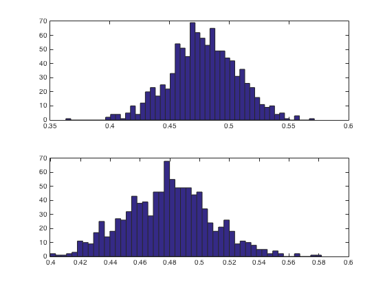
figure
subplot(2,1,1)
hist(m1,50)
subplot(2,1,2)
hist(m2,50)
mean(m1)
mean(m2)
std(m1)
std(m2)

y =
    0.0076
    0.1253
    0.7569
    0.2094
    0.4729
    0.0316
    0.9912
    0.2786
    0.8140
    0.4911
    0.3587
    0.4710
    0.4195
    0.5091
    0.6741
    0.7100
    0.4897
    0.5014
    0.0007
    0.3830
    0.3474
    0.6258
    0.9185
    0.9014
    0.6600
    0.8927
    0.0038
    0.4455
    0.5090
    0.3830
    0.7089
    0.6247
    0.8909
    0.2380
    0.0854
    0.1631
    0.0758
    0.4118
    0.4839
    0.6714
    0.1564
    0.6374
    0.5745
    0.5900
    0.2622
    0.9397
    0.6651
    0.8160
    0.7631
    0.8537
    0.6834
    0.9245
    0.8710
    0.1642
    0.9891
    0.1098
    0.1353
    0.9855
    0.0413
    0.5222
    0.1700
    0.9170
    0.2860
    0.6094
    0.3714
    0.0693
    0.5561
    0.0323
    0.4145
    0.8976
    0.5232
    0.2807
    0.2814
    0.5201
    0.3245
    0.4115
    0.6242
    0.6617
    0.3796
    0.6700
    0.8352
    0.0667
    0.4345
    0.1021
    0.0417
    0.3144
    0.2083
    0.9490
    0.7538
    0.7655
    0.1035
    0.5466
    0.5532
    0.0749
    0.8732
    0.1990
    0.2426
    0.6686
    0.6568
    0.1033
ans =
    0.4784
ans =
    0.4791
ans =
    0.0282
ans =
    0.0288

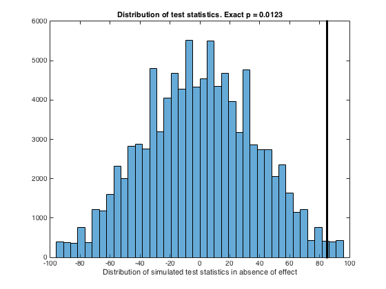
4 Comparing means with permutation tests

%We stress out a rat for 2 weeks
%We then take out 10 neurons
%5 we treat with Ketamine and 5 we don't treat at all
%We then count the number of dendritic spines of each neuron
%Hypothesis: Ketamine works by growing dendritic spines

%Why do permutation tests?
%p value of an ANOVA or t-test (or similar tests) is only exact for
%specific distributions. If the distribution of the data deviates, p value
%might be off. In contrast, permutation tests are distribution free.
%We use the data itself to approximate the distribution. As long as the
%sample data is representative of the population it came from, there is no
%problem.

K = [117 123 111 101 121] %Number of dendritic spines in Ketamine treated neurons
%K = [98 104 106 92 88] %Number of dendritic spines per control neuron
C = [98 104 106 92 88] %Number of dendritic spines per control neuron

numMCS = 1e5; %Number of Monte Carlo simulations
nK = length(K); %Number of Ketamine treated neurons
nC = length(C); %Number of control neurons

%Step 1 in this process: Come up with a reasonable test statistic
testStatistic = sum(K)-sum(C)
%This is perhaps the point that will require the most thought in the future
%As you use this. Coming up with a reasonable test statistic. It depends on
%your hypothesis. This could be one-tailed or two-tailed or whatever.

%What do we want to know about the test statistic in order to evaluate our
%hypothesis that Ketamine is effective in growing dendritic spines?

%How likely a value of 85 (the value we got) is by chance alone.
%We permute the values and draw groups arbitrarily (randomly) and see what
%values of the test statistic we get. Doing this a large number of times
%allows us to create a "noise distribution" of the test statistic.
%Logic: If there is no effect of the Ketamine, it should not matter which group the neurons
%came from.

dTS = zeros(numMCS,1); %Initialize and preallocate the distribution of the test statistic
allData = [K C]; %Concatenate all the data

%Monte Carlo method: Random permutation/rearrangement of the group labels
for ii=1:numMCS %However many times you want to do this
    indices = randperm(nK+nC); %Rejigger indices
    %Critical difference: Instead of drawing with replacement, we
    %rearrange. Each index only shows up once at any given time
    tempDATA = allData(indices); %Create a newly permuted dataset. We now carve that into groups
    group1 = tempDATA(1:nK); %Capture the first n elements
    tempDATA(:,1:nK) = []; %Delete those from the permuted dataset
    group2 = tempDATA; %Group 2 is simply what is left (the remaining data of the 2nd group)
    dTS(ii) = sum(group1)-sum(group2); %Capture the simulated test statistic for each run
end

figure
histogram(dTS,40)

%Finding the exact p value
exactP = sum((dTS>=testStatistic))/length(dTS); %One tailed!
%Out of curiosity: Two tailed
%exactP = sum(testStatistic<=abs(dTS))/length(dTS); %Two tailed case

%Add some labels
line([testStatistic testStatistic],[min(ylim) max(ylim)],'color','k','linewidth',3)
xlabel('Distribution of simulated test statistics in absence of effect')
title(['Distribution of test statistics. Exact p = ', num2str(exactP,'%1.4f')])

%Philosophical considerations
%The "exact" p value is given this data, but losing the labels, randomly
%drawing numMCS times. So what does this mean? What is this is a
%distribution of?
%And how exact is it?

K =
   117   123   111   101   121
C =
    98   104   106    92    88
testStatistic =
    85

Published with MATLAB® R2015a