Contents

%This lab introduces the notion of simulation to calculate power

1 Init Start with a blank slate

clear all
close all
clc

%Seed the random number generator
s = RandStream('mt19937ar','Seed',sum(round(clock)));
RandStream.setGlobalStream(s);

2 p values, mean differences and significance

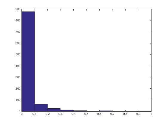
sampleSize = 253; %This will control our sample size
numRep = 1e3; %This is the number of times we draw randomly
meanDifference = 0.25; %This will control the actual difference in means in the population

A = randn(numRep,sampleSize,1); %Draw from a random normal distribution with zero mean
A(:,:,2) = randn(numRep,sampleSize,1) + meanDifference; %Similar
%But with an average mean difference

for ii = 1:numRep
    [H(ii) P(ii)] = ttest2(A(ii,:,1),A(ii,:,2));
    %Test 1st sheet vs. 2nd sheet with a 2 sample t-test
end

sum(H)
figure
hist(P)

ans =
   798

3 PPV - "positive predictive value"

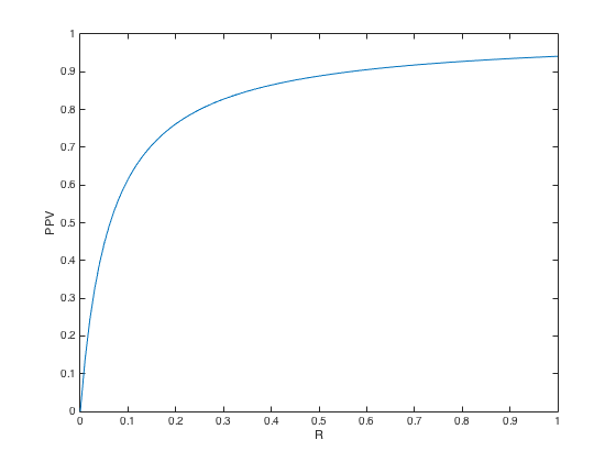
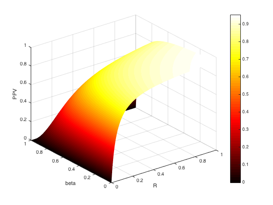
%The posterior probability that if something is significant, it is true

%1 Case
alpha = 0.05; %Classic choice
beta = 0.2; %Classic choice - power is 1-beta, we aim for 0.8
R = 0.5; %Whatever - reasonable choice
PPV = ((1-beta)*R)/(R-beta*R+alpha)

%2 All Rs from 0 to 1
R = 0:0.01:1; %Now, let's let R go from 0 to 1
for ii = 1:length(R)
    PPV(ii) = ((1-beta)*R(ii))/(R(ii)-beta*R(ii)+alpha);
end
figure
plot(R,PPV)
xlabel('R')
ylabel('PPV')

%3 So far, we "clamped" power at 0.8 - what if we had lower power?
%Why might we have lower power?
%Because it is hard to get high power if the effect size is low.
%Who has the funds to recruit thousands of participants?
beta = 1:-0.01:0; %Power = 1 - beta, so we'll have this go from 1 to 0
for ii = 1:length(R)
    for jj = 1:length(beta)
    PPV(ii,jj) = ((1-beta(jj))*R(ii))/(R(ii)-beta(jj)*R(ii)+alpha);
    end
end

%Let's summarize the entire Ioannidis paper in one figure
%linking power, R and PPV
figure
h = surf(R,beta,PPV); %Make a surface plot
set(h,'linestyle','none') %Take the mesh off
set(h,'facecolor','interp') %Interpolate colors
xlabel('R')
ylabel('beta')
zlabel('PPV')
colorbar
colormap('hot')

PPV =
    0.8889

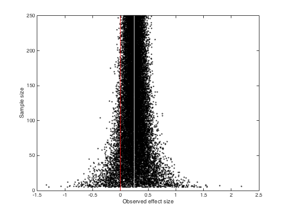
4 Funnel plots

%Funnel plots are a meta-analyic tool. They effectivly plot effect size
%vs. power.
%As you increase power, the effects cluster around the "real" effect
%Like in a funnel. Hence funnel plot

%There are more things to see in funnel plots.
%We'll write them here once we did a couple.
%But let's first develop them.

sampleSize = 5:250; %In the interest of time.
effectSize = 0.25; %Later, we put in a real effect size
repeats = 1e2; %I want to save time in class. We do a 100 repeats per sample size

%Preallocate
%This will contain the mean differences - we do a nested loop. To save
%time, we preallocate it in memory.
meanDifference = zeros(length(repeats),length(sampleSize));

%Calculations
%This will allow us to simulate the observed effect sizes for a given
%power. Doing so rr number of times, which will allow us to assess the
%spread
for rr = 1:repeats %Going through all the repeats
    for ii = 1:length(sampleSize) %Going through all the sample sizes
        A = randn(sampleSize(ii),1) + effectSize; %Drawing from a random normal distribution plus effectsize
        B = randn(sampleSize(ii),1); %Doing it again
        meanDifference(rr,ii) = mean(A)-mean(B); %Calculating the actual mean difference and putting it in the storage structure
    end
end

%To plot this, it is easiest to linearize it first
%We could plot this in a for loop as well, but this is exhausting
%So let's not do that. Instead, let's linearize first

linearizedMeanDifference = meanDifference(:); %Put it all in one vector
temp = repmat(sampleSize,[repeats 1]); %Tile the sample size
linearizedsampleSize = temp(:); %Same for sample size

figure
plot(linearizedMeanDifference,linearizedsampleSize,'.','color','k')

ylabel('Sample size')
xlabel('Observed effect size')
set(gcf,'color','w')

line([0 0], [0 max(ylim)],'color','r') %No effect
line([effectSize effectSize], [0 max(ylim)], 'color', 'w') %Real effect

Published with MATLAB® R2015a