Contents
%In this lab, we will do processing of LFP traces in the time domain
%and 2D convolution.

%1 Init - Clear workspace and load data

clear all
close all
clc
%Load data - whatever your directory is.
load('/Users/lascap/Desktop/Old Desktop/Work/Teaching/Fall 2016/Math Tools 2016/LAB/LFPdata.mat');
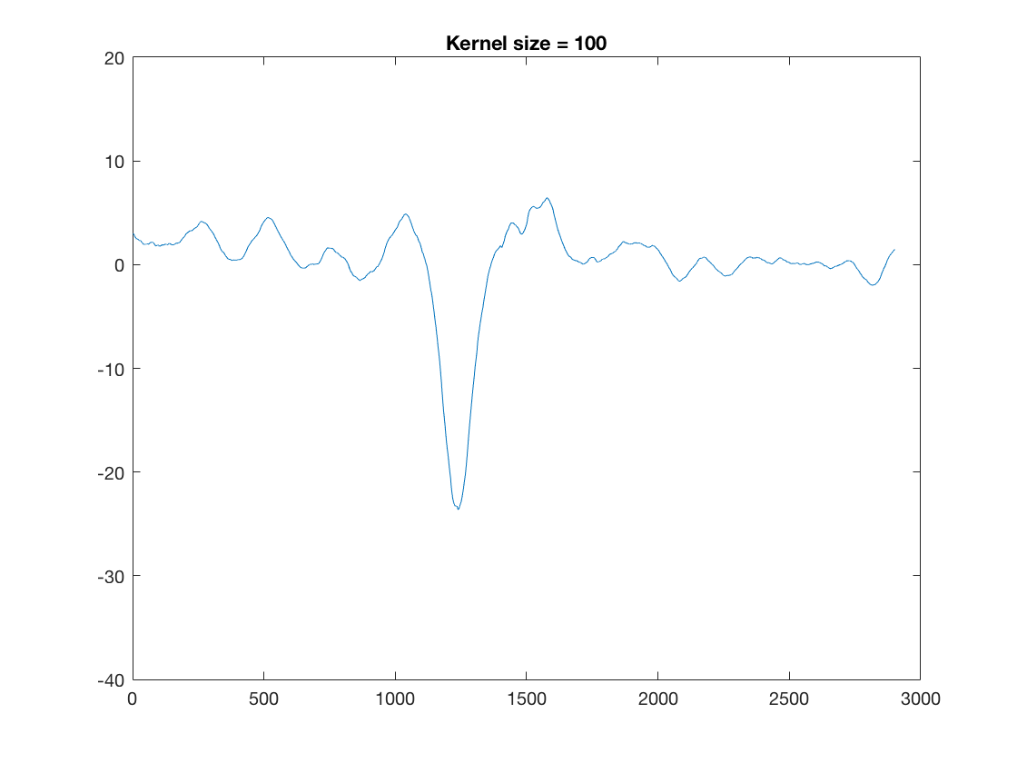
%Exploratory data analysis - plotting the raw data and doing 1D convolution
figure
plot(A)
for ii = 1:100;
kernelSize = ii; %This is the length of our kernel
kernel = ones(kernelSize,1); %Symmetric, equal weight kernel of size kernelSize
pause(0.25)
Aconv = conv(A,kernel,'valid')./sum(kernel); %If we don't normalize by sum of kernelweights, result will depend on size of kernel
plot(Aconv)
title(['Kernel size = ', num2str(ii)])
ylim([-40 20])
shg
end
%xlim([0 3000])
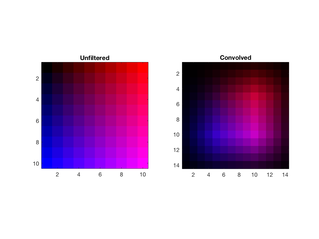
2D convolution - before we do this with actual image data (where there is a lot going on)
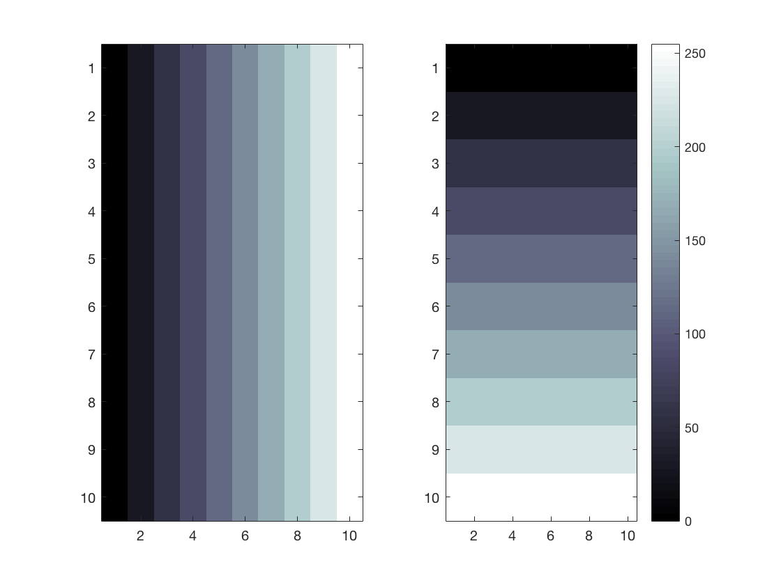
%let's do this with an artificial image where it is easy to see what
%convolution is doing.

%1. Let's create luminance ramps
clear IM

numSteps = 10; %I want n steps
stepSize = linspace(0,255,numSteps); %MATLAB represents luminance as a number from 0 to 255
%For space reasons, mostly - 8 bit = 1 byte. 256 states
[x,y] = meshgrid(0:stepSize(2):255,0:stepSize(2):255); %Creating luminance ramps with meshgrid

%Meshgrid creates ramps. To wit
figure
subplot(1,2,1)
imagesc(x)
subplot(1,2,2)
imagesc(y)
colorbar
colormap(bone) %To highlight that this represents luminance

%We use these ramps to create an image matrix IM
IM(:,:,1) = uint8(x); %The first sheet of IM - a 3d matrix - will be x - Red
IM(:,:,2) = uint8(zeros(length(x))); %Make the green channel all zeros
IM(:,:,3) = uint8(y); %Same for blue

figure
subplot(1,2,1)
image(IM)
axis square
title('Unfiltered')

kernel = ones(5);
convIM = uint8(round(convn(IM,kernel))./sum(sum(kernel)));
subplot(1,2,2)
image(convIM)
axis square
title('Convolved')
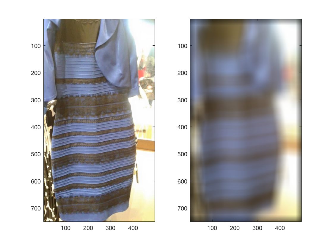
Doing image processing of an actual image
dress = imread('thedress.jpg'); %Putting the dress into a matrix
figure
image(dress)
axis equal
shg
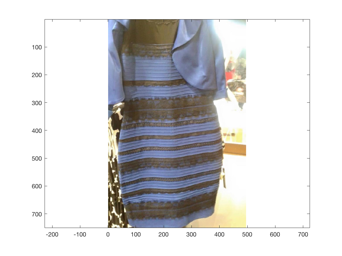
That is the raw dress. We now convolve the image
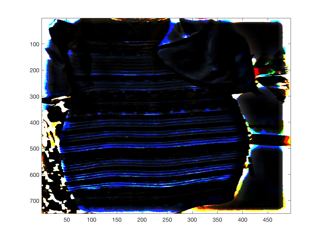
kernelWidth = 50;
figure
subplot(1,2,1)
image(dress)
subplot(1,2,2)
kernel = ones(kernelWidth);
lp = uint8(convn(dress,kernel,'same')./sum(sum(kernel))); %Same makes a lot of sense for image processing
%because we usually want to do further processing, e.g. edge detection
image(lp)

hp = dress-lp; %This an image that contains a subtracted version of the low pass.
%We can only subtract if dress and lp are the same size, which is why we
%convolved with "same" above. But note that we used a simple kernel.
figure
image(hp)

%Edge enhancement
temp = find(hp>50); %Anywhere where there is signal above threshold
hp(temp) = 255; %Set it to full
image(hp)


%Assignment (small group): Add a edge handling option to your MATLAB -
%either constant, reflectance or circular.
%Do this now, in small group.
%Zero padding is literally a failure of imagination. It is unlikely that
%the image (in the real world) ends where you happened to take it.