Contents

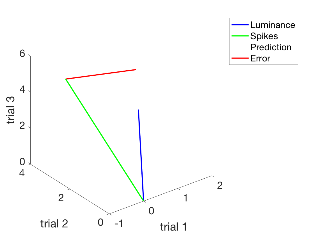
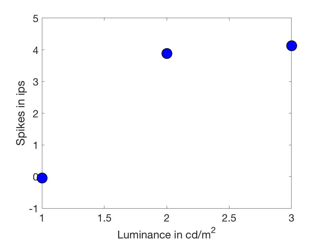
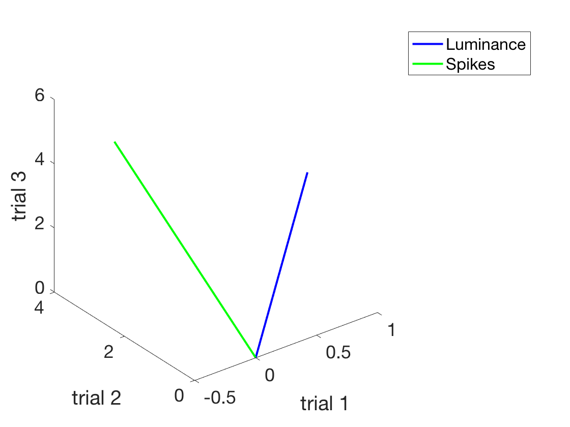
clear all
close all

xLuminance = [1:3]'; %A column vector of IV in cd/m^2
ySpikes = 1.5*xLuminance + 0.5 + randn(length(xLuminance),1).*2; %Noisy integrate and fire

%Make a nice plot of the situation
figure
h = plot(xLuminance,ySpikes,'o') %First use of an object handle!
set(h,'Markersize',18)
h.MarkerFaceColor = 'b';
h.MarkerEdgeColor = 'k';
xlabel('Luminance in cd/m^2')
ylabel('Spikes in ips')
set(gca,'fontsize',18)

%This is legit, but to see how the equation (which works) works
%let's look at this graphically. Or geometrically.
%To do that, we need to express the experiment visually.
%Now, each trial is a dimension.
figure
h1 = plot3([0, xLuminance(1)], [0, xLuminance(2)], [0, xLuminance(3)])
h1.Color = 'b';
h1.LineWidth = 2;
hold on
h2 = plot3([0, ySpikes(1)], [0, ySpikes(2)], [0, ySpikes(3)])
h2.Color = 'g';
h2.LineWidth = 2;
legend('Luminance','Spikes')
xlabel('trial 1')
ylabel('trial 2')
zlabel('trial 3')
set(gca,'fontSize',18)
rotate3d on

h = 
  Line with properties:

              Color: [0 0.447 0.741]
          LineStyle: 'none'
          LineWidth: 0.5
             Marker: 'o'
         MarkerSize: 6
    MarkerFaceColor: 'none'
              XData: [1 2 3]
              YData: [-0.0428433530388914 3.88022557987611 4.13042332294946]
              ZData: [1x0 double]

  Use GET to show all properties
h1 = 
  Line with properties:

              Color: [0 0.447 0.741]
          LineStyle: '-'
          LineWidth: 0.5
             Marker: 'none'
         MarkerSize: 6
    MarkerFaceColor: 'none'
              XData: [0 1]
              YData: [0 2]
              ZData: [0 3]

  Use GET to show all properties
h2 = 
  Line with properties:

              Color: [0.85 0.325 0.098]
          LineStyle: '-'
          LineWidth: 0.5
             Marker: 'none'
         MarkerSize: 6
    MarkerFaceColor: 'none'
              XData: [0 -0.0428433530388914]
              YData: [0 3.88022557987611]
              ZData: [0 4.13042332294946]

  Use GET to show all properties

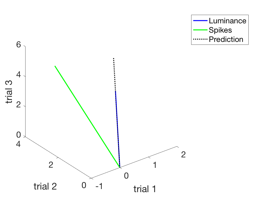
Now, let's actually use the formula we derived

beta = (ySpikes' * xLuminance)/(xLuminance'*xLuminance) %Find the beta
beta = dot(ySpikes,xLuminance)/dot(xLuminance,xLuminance) %Same if you don't remember which is which
prediction = beta*xLuminance %Make a prediction (simplest possible)
%Add this to the plot - the plot thickens
h3 = plot3([0, prediction(1)], [0, prediction(2)], [0, prediction(3)]);
set(h3,'linewidth',2)
set(h3,'linestyle',':')
h3.Color = 'k'
legend('Luminance','Spikes','Prediction')
shg

beta =
          1.43634841254012
beta =
          1.43634841254012
prediction =
          1.43634841254012
          2.87269682508024
          4.30904523762036
h3 = 
  Line with properties:

              Color: [0 0 0]
          LineStyle: ':'
          LineWidth: 2
             Marker: 'none'
         MarkerSize: 6
    MarkerFaceColor: 'none'
              XData: [0 1.43634841254012]
              YData: [0 2.87269682508024]
              ZData: [0 4.30904523762036]

  Use GET to show all properties

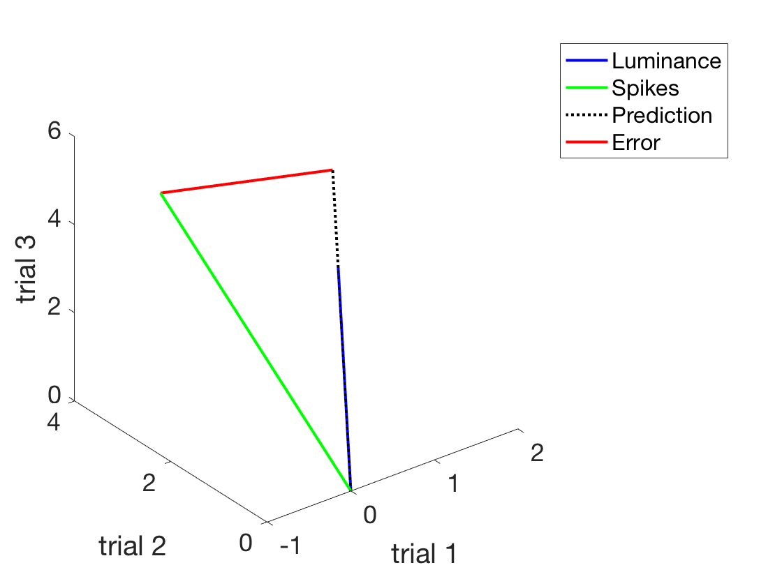
Let's explicitly add the distance between the two

h4 = plot3([ySpikes(1), prediction(1)], [ySpikes(2), prediction(2)], [ySpikes(3), prediction(3)]);
set(h4,'linewidth',2)
set(h4,'linestyle','-')
h4.Color = 'r'
legend('Luminance','Spikes','Prediction','Error')
shg

h4 = 
  Line with properties:

              Color: [1 0 0]
          LineStyle: '-'
          LineWidth: 2
             Marker: 'none'
         MarkerSize: 6
    MarkerFaceColor: 'none'
              XData: [-0.0428433530388914 1.43634841254012]
              YData: [3.88022557987611 2.87269682508024]
              ZData: [4.13042332294946 4.30904523762036]

  Use GET to show all properties

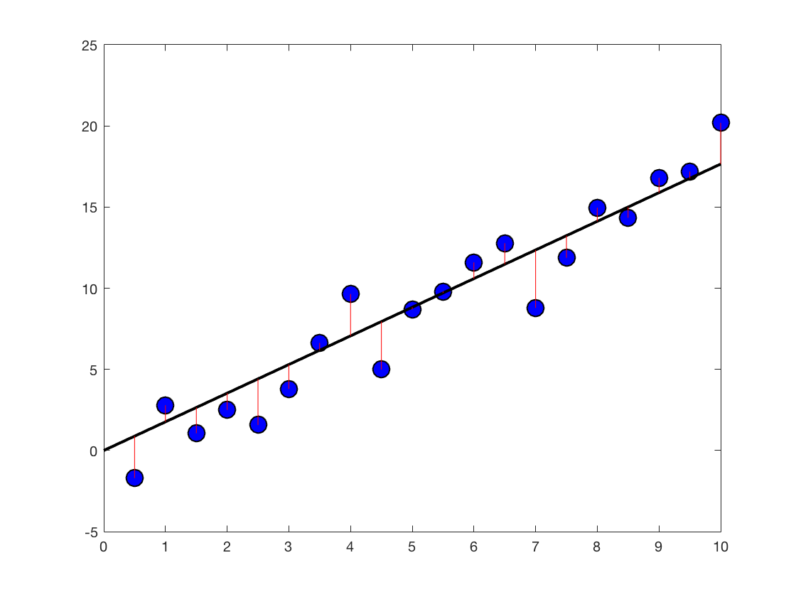
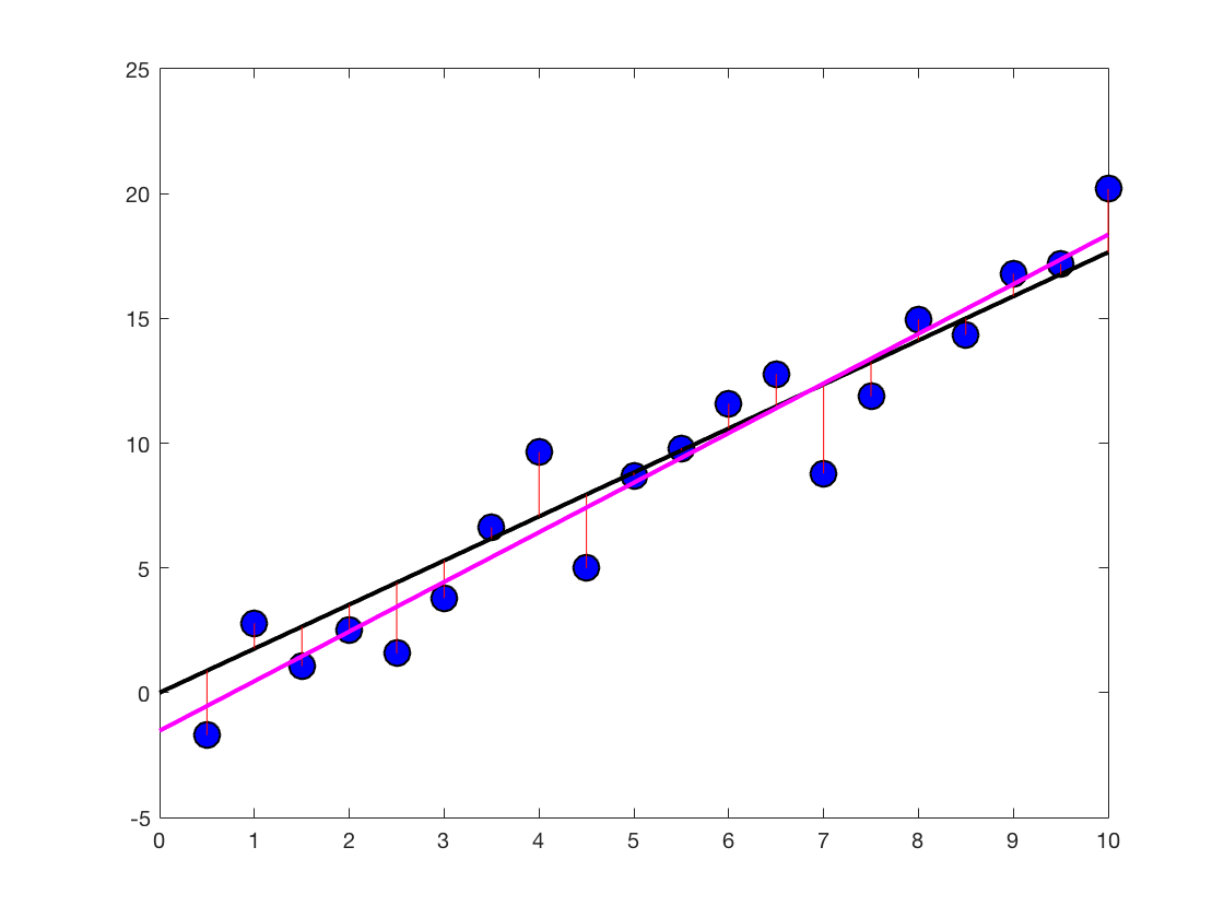
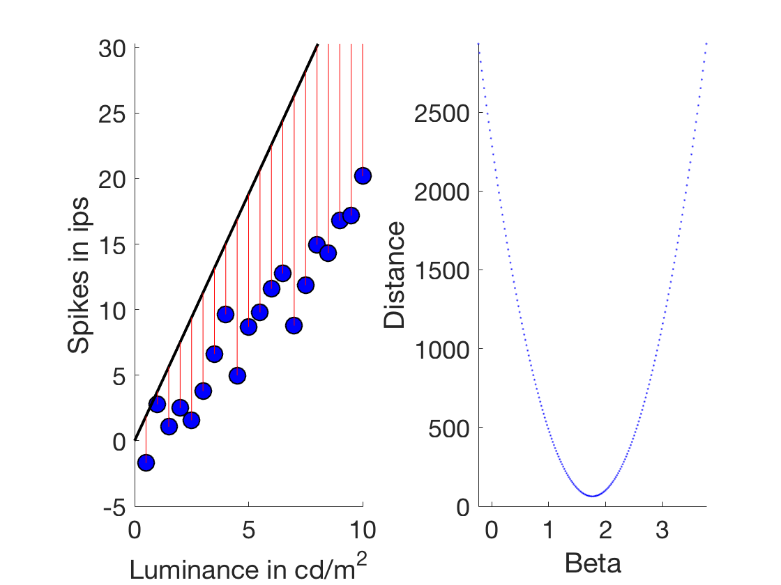
Now that we convinced ourselves that this is in fact the correct beta (geometrically)

we can go back and plot the solution We could open the old figure again, but let's start from scratch What if we had 20 measurements (20 trials)?

maxLuminance = 10;
xLuminance = [0.5:0.5:maxLuminance]'; %A column vector of IV in cd/m^2 - 20 luminance values
ySpikes = 1.5*xLuminance + 0.5 + randn(length(xLuminance),1).*2; %Noisy integrate and fire
beta = dot(ySpikes,xLuminance)/dot(xLuminance,xLuminance) %Same if you don't remember which is which
prediction = beta*xLuminance %Make a prediction (simplest possible)
figure
h4 = plot(xLuminance,ySpikes,'o')
set(h4,'Markersize',12)
h4.MarkerFaceColor = 'b';
h4.MarkerEdgeColor = 'k';
pause
hold on
regressionLineX = linspace(0,maxLuminance,10); %Gives us 10 equally spaced numbers between 0 and 4. Intrapolation, x-base
regressionLineY = beta .* regressionLineX; %Find the ys of the regression line

h5 = plot(regressionLineX,regressionLineY,'k')
set(h5,'linewidth',2)
pause
%h6 = plot(xLuminance,prediction,'o')
%set(h6,'Markersize',18)
%h6.MarkerFaceColor = 'k';
%h6.MarkerEdgeColor = 'y';
lh = line([xLuminance'; xLuminance'],[prediction'; ySpikes'], 'color','r');

pause

beta =
          1.76497701782015
prediction =
         0.882488508910077
          1.76497701782015
          2.64746552673023
          3.52995403564031
          4.41244254455039
          5.29493105346046
          6.17741956237054
          7.05990807128062
           7.9423965801907
          8.82488508910077
          9.70737359801085
          10.5898621069209
           11.472350615831
          12.3548391247411
          13.2373276336512
          14.1198161425612
          15.0023046514713
          15.8847931603814
          16.7672816692915
          17.6497701782015
h4 = 
  Line with properties:

              Color: [0 0.447 0.741]
          LineStyle: 'none'
          LineWidth: 0.5
             Marker: 'o'
         MarkerSize: 6
    MarkerFaceColor: 'none'
              XData: [1x20 double]
              YData: [1x20 double]
              ZData: [1x0 double]

  Use GET to show all properties
h5 = 
  Line with properties:

              Color: [0 0 0]
          LineStyle: '-'
          LineWidth: 0.5
             Marker: 'none'
         MarkerSize: 6
    MarkerFaceColor: 'none'
              XData: [1x10 double]
              YData: [1x10 double]
              ZData: [1x0 double]

  Use GET to show all properties

Multiple regression - simplest case: Adding a constant to the regression equation

%Even having more than one predictor makes it a multiple regression, even
%if it is a constant.

%We need to represent the baseline
%We need as many baselines as there are trials, and it always should have
%the same value. Because we assume this is a constant
baseline = ones(length(xLuminance),1)

designMatrix = [xLuminance, baseline];
betas = pinv(designMatrix' * designMatrix) * designMatrix'*ySpikes; %We should get a vector of 2 betas out of this
prediction = designMatrix*betas;

baseline =
     1
     1
     1
     1
     1
     1
     1
     1
     1
     1
     1
     1
     1
     1
     1
     1
     1
     1
     1
     1

Let's plot the new regression line on top of the old figure

regressionLineYBar = betas(1)*regressionLineX + betas(2) ...
    * ones(1,length(regressionLineX));
plot(regressionLineX,regressionLineYBar,'color','m','linewidth',2)


pause

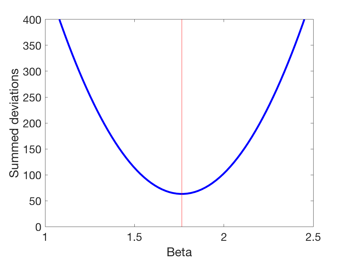
Dropping marbles - which beta is the right beta?

beta
%Let's explore the space of betas
startExploration = beta-2;
endExploration = beta+2;
numBeta = 200;
testBetas = linspace(startExploration,endExploration,numBeta) ;%200 betas between the actual beta and +/- 2
%Let's just go through them and try them
for ii = 1:numBeta
    prediction = testBetas(ii).*xLuminance; %Do this numBeta times
    %We now need to introduce a distance metric
    %We start with sum of squares (the most common maybe)
    distanceSum(ii) = sum((prediction-ySpikes).^2); %Sum of squares
   % distanceSum(ii) = sum((prediction-ySpikes)); %Simple summed deviations
    %distanceSum(ii) = sum(log(prediction-ySpikes)); %Absolute summed deviations
end

%Let's plot that
figure
plot(testBetas,distanceSum,'b','linewidth',3)
%We also want to indicate with a line where the original beta was
line([beta beta], [min(ylim) max(ylim)], 'color','r')
xlabel('Beta')
ylabel('Summed deviations')
set(gca,'fontsize',18)
set(gcf,'color','w')
ylim([0 400])

beta =
          1.76497701782015

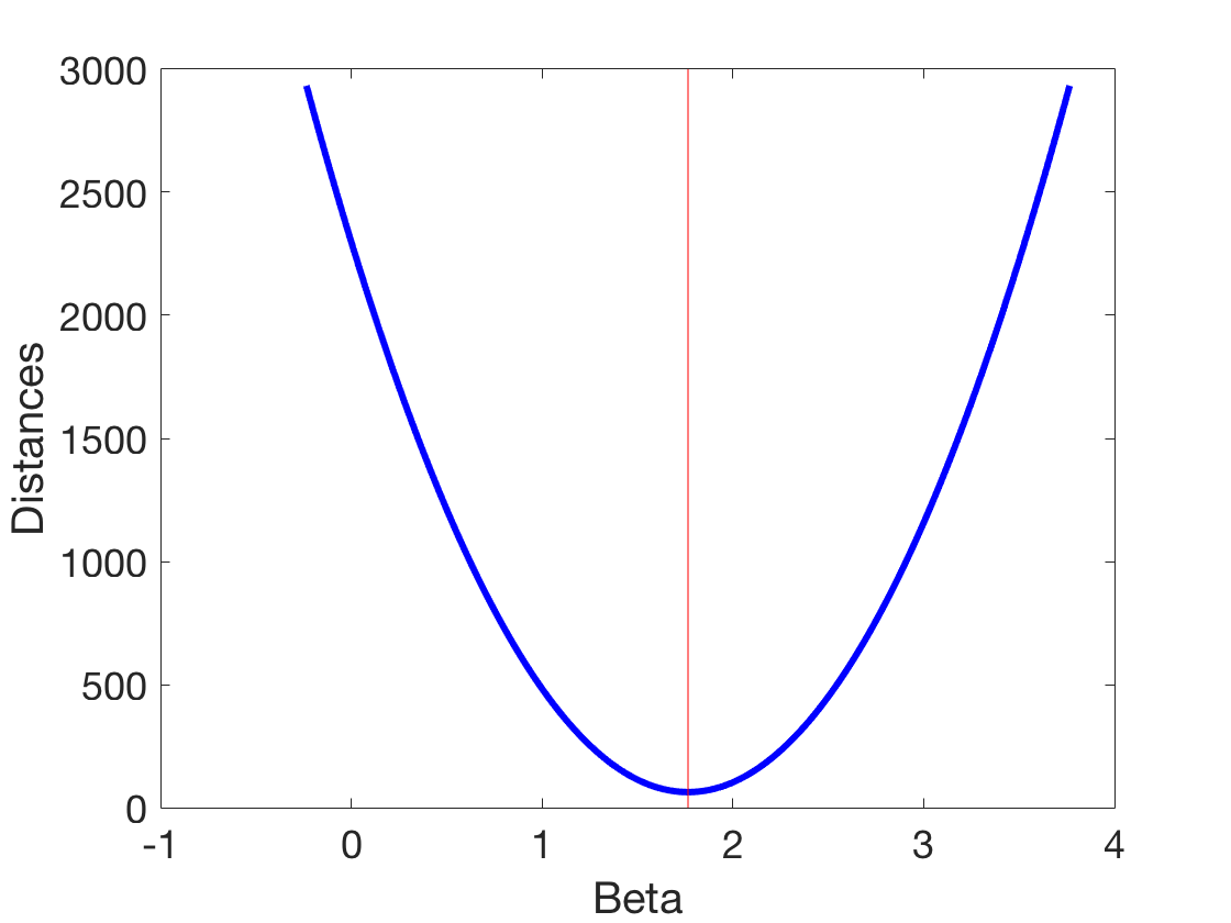
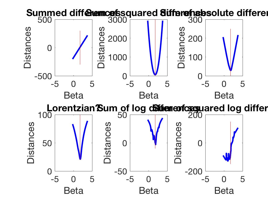
Going deeper into optimization - and gradient descent

beta
startExploration = beta-2;
endExploration = beta+2;
testBetas = linspace(startExploration,endExploration,200);
for ii = 1:length(testBetas)
    prediction(:,ii) = testBetas(ii)*xLuminance;
    distanceSum(1,ii) = sum(prediction(:,ii)-ySpikes); %Simple
    distanceSum(2,ii) = sum((prediction(:,ii)-ySpikes).^2); %Squared
    distanceSum(3,ii) = sum(abs(prediction(:,ii)-ySpikes)); %Absolute value
    distanceSum(4,ii) = sum(log(1 + (prediction(:,ii)-ySpikes).^2)); %Lorentzian
    distanceSum(5,ii) = sum(log(prediction(:,ii)-ySpikes)); %Weirdness
    distanceSum(6,ii) = sum(log(prediction(:,ii)-ySpikes).^2); %Weirdness

end

figure
plot(testBetas,distanceSum(2,:),'b','linewidth',3)
line([beta beta],[min(ylim) max(ylim)],'color', 'r')
xlabel('Beta')
ylabel('Distances')
set(gca,'fontsize',18)

figure
for ii = 1:6
    subplot(2,3,ii)
plot(testBetas,distanceSum(ii,:),'b','linewidth',3)
line([beta beta],[min(ylim) max(ylim)],'color', 'r')
xlabel('Beta')
ylabel('Distances')
if ii == 1
    title('Summed differences')
elseif ii == 2
    title('Sum of squared differences')
elseif ii == 3
    title('Sum of absolute differences')
elseif ii == 4
    title('Lorentzian?')
elseif ii == 5
    title('Sum of log differences')
elseif ii == 6
    title('Sum of squared log differences')

end

set(gca,'fontsize',18)

end
set(gcf,'color','w')

beta =
          1.76497701782015
Warning: Imaginary parts of complex X and/or Y arguments ignored 
Warning: Imaginary parts of complex X and/or Y arguments ignored 

Gradient descent revisited

figure
for ii = 1:length(testBetas)
    subplot(1,2,1)
    hold on
    prediction = testBetas(ii)*xLuminance;
    h7 = plot(xLuminance, ySpikes, 'o');
    set(h7,'markersize',12)
    set(h7,'markerfacecolor','b')
    set(h7,'markeredgecolor','k')
    xlabel('Luminance in cd/m^2')
    ylabel('Spikes in ips')
    set(gca,'fontsize',18)
    regressionLineX = linspace(0,10,100); %Intrapolate

    regressionLineY = testBetas(ii) * regressionLineX;
    h8 = plot(regressionLineX, regressionLineY, 'k');
    set(h8,'linewidth',2);

for jj = 1:length(ySpikes)
  h(jj) = line([xLuminance(jj) xLuminance(jj)],[prediction(jj) ySpikes(jj)],'color','r');
end
    ylim([-5 1.5*max(ySpikes)])
    subplot(1,2,2)
    hold on
    plot(testBetas(ii),distanceSum(2,ii),'.','color','b','linewidth',3)
    xlabel('Beta')
    ylabel('Distance')
    set(gca,'fontsize',18)
    xlim([startExploration endExploration])
    ylim([0 max(distanceSum(2,:))])
    shg
    pause(0.1)
    if ii < length(testBetas)
    delete(h8)
    delete(h)
    end
end

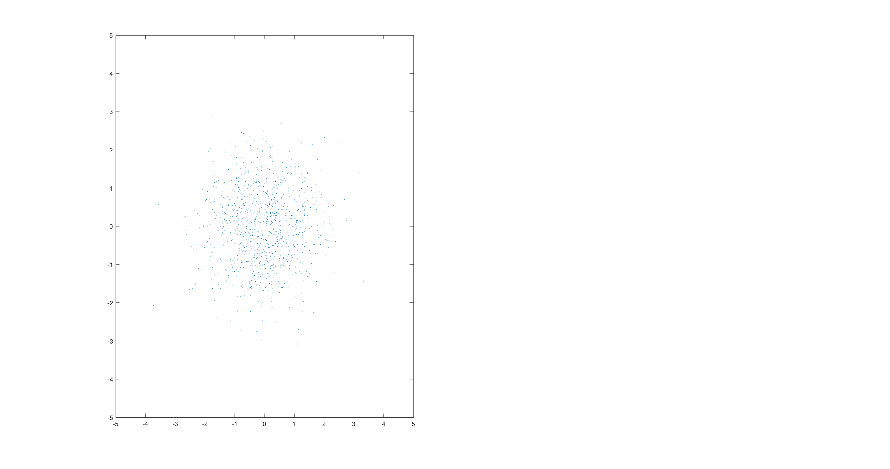
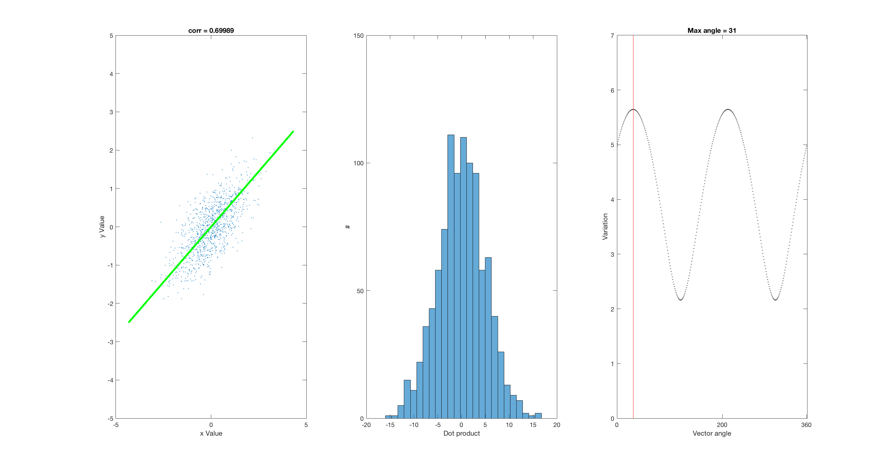
PCA

corr = 0.7 %Possible values: 0, 0.7, 0.9, 0.3, -0.7
A = randn(1000,2); %uncorrelated data

if corr == 0.7 % Corr ~ 0.7
B = randn(1000,1);
C = randn(1000,1);
D = (B + C)./2; %correlated data (B and D)
elseif corr == 0
B = randn(1000,1);
D = randn(1000,1);
elseif corr == 0.9
B = randn(1000,1);
C = randn(1000,1);
D = (3.*B + C)./4; %correlated data (B and D)
elseif corr == 0.3
Q = randn(1000,1);
B = randn(1000,1);
C = randn(1000,1);
D = ((3*Q) + B + C)./5; %correlated data (B and D)
elseif corr == -0.7
B = randn(1000,1);
C = randn(1000,1);
D = (B + C)./2; %correlated data (B and D)
D = D.*-1;
end

dotVec = [B,D];
dotProducts = zeros(1000,1);
spreads = zeros(360,1);

fullScreen
subplot(1,2,1)
plot(A(:,1),A(:,2),'.')
xlim([-5 5])
ylim([-5 5])

fullScreen
subplot(1,3,1)
plot(B(:,1),D(:,1),'.')
xlabel('x Value')
ylabel('y Value')
temp = corrcoef(B,D);
title(['corr = ', num2str(temp(1,2))])
xlim([-5 5])
ylim([-5 5])
M = [5;0];
hold on
plotv(M,':');
plotv(-1.*M,':');
h = findobj('linestyle',':');
set(h,'color','r')
set(h,'linestyle','-')
for ii = 1:1000
    dotProducts(ii,1) = dot(dotVec(ii,:),M);
end

subplot(1,3,2)
histogram(dotProducts,25)
xlabel('Dot product')
ylabel('#')
xlim([-20 20])
ylim([0 150])


subplot(1,3,3)
plot(1,std(dotProducts),'.','color','k');
xlabel('Vector angle')
ylabel('Variation')
xlim([0 361])
ylim([0 7])
set(gca,'XTick', [0 200 360])
hold on
%set(h,'color','r')
%columnVector = [-5 5]'
%hold on

pause
%R = [0 -1; 1 0];
for aa = 1:360
subplot(1,3,1)
angle = deg2rad(aa);
R = [cos(angle) -sin(angle); sin(angle), cos(angle)];
RM = R*M;
set(h,'linestyle','none')
plotv(RM,':');
plotv(-1.*RM,':');
h = findobj('linestyle',':');
set(h,'color','r')
set(h,'linestyle','-')
pause(0.005)

for ii = 1:1000
    dotProducts(ii,1) = dot(dotVec(ii,:),RM);
end

subplot(1,3,2)
histogram(dotProducts,25)
xlabel('Dot product')
ylabel('#')
xlim([-20 20])
ylim([0 150])

subplot(1,3,3)
spreads(aa) = std(dotProducts);
plot(aa,spreads(aa),'.', 'color','k');
xlabel('Vector angle')
ylabel('Variation')
set(gca,'XTick', [0 200 360])

hold on
%columnVector2 = R*columnVector;
%plot(columnVector2,'color','r')
%myVector = [-5 0; 5 0]l
%myVector2 = R*myVector;
%line(myVector(:,1),myVector(:,2),'color','r')
%pause
%line(myVector2(:,1),myVector2(:,2),'color','b')
end
maxSpreads = max(spreads);
temp = find(spreads == maxSpreads);
title(['Max angle = ', num2str(temp(1))])
line([temp(1) temp(1)],ylim,'color','r')

subplot(1,3,1)
M = [5;0];
angle = deg2rad(temp(1,1)-1);
R = [cos(angle) -sin(angle); sin(angle), cos(angle)];
RM = R*M;
set(h,'linestyle','none')
plotv(RM,':');
plotv(-1.*RM,':');
h = findobj('linestyle',':');
set(h,'color','g')
set(h,'linestyle','-')
set(h,'linewidth',3)

corr =
                       0.7

Published with MATLAB® R2016a