Contents
%Lab 3: Functions, SVD, error correction, Vectorization, Saving and Loading
1 Functions
%Functions made: Width and deg2rad

%Exercise 1: Make a rad2deg function
%Exercise 2: Package the inner product logic we wrote last time into a
%function
%Exercise 3: Package the matrix multiplication logic from lab 2 into a
%function
2 SVD! The most useful thing (for us) in Linear Algebra
%a) Verify the 3 things I so boldly asserted last week.
%Remember: We did not derive or prove this. So let's at least check them

for ii = 1:1%e5 %Let's try 100,000 times. To see if the SVD always works
M = randn(2,2) %Create some random matrix M. Any matrix will do. This will represent the operations
x = randn(2,2) %Create some random matrix x that represents data.
[U,S,V] = svd(M) %Do the SVD on matrix M.

C = M*x %To find out what the operations matrix does to the data, apply it

%Check whether SVD of M and M do correspond to the same thing?
D = U * S * V' * x

%The other radical claim was that the SVD corresponds to a sum of outer
%products. Let's convince ourselves that this is actually true. What if I
%forgot a sign somewhere?
SOP = (S(1,1).*(U(:,1)*V(:,1)')*x) + ...
    (S(2,2).*(U(:,2)*V(:,2)')*x)

%We convinced ourselves by visual inspection that the SVD and M indeed
%produce the same output. Generally speaking, that is not good enough - we
%want to do this programmatically.

C == D;

%The problem with this is that MATLAB has enough numerical precision
%to get you in trouble. It's not infinite, so it's not perfect, but there
%are slight rounding errors somewhere in the 16th after-digit place
%So we need to set the numerical precision we want

%Setting numerical precision:
C = round(C.*1000)./1000; %Setting numerical precision to 3 after comma digits
%This works by multiplying by thousand, rounding, then dividing by 1000
%again. This might make a good function. Because you will want to
%set the precision arbitrarily, user-defined. And you will use this a lot.
%And it is clunky.
D = round(D.*1000)/1000;

C == D;

%This is nice, but still requires visual inspection.
%How do we reduce this output to a single number that tells
%me whether it matches or not?

%Idea: Let's sum them up and compare to the number of elements in the
%matrix

E(ii) = sum(sum(C == D)) == numel(C); %This presumes that C and D are
%the same dimensionality, because we only check C.
end

%Exercise for the reader:
%Do this with matrices of different dimensionalities
%Convince yourself programmatically that SOP also corresponds to the others
%I did this just for one case
%Write a numerical precision function
M =
      -1.5176      0.50836
      -2.1421      0.39312
x =
       0.3078      -1.3729
       1.3686      0.67888
U =
     -0.59101     -0.80667
     -0.80667      0.59101
S =
       2.6966            0
            0      0.18259
V =
      0.97342     -0.22902
     -0.22902     -0.97342
C =
      0.22863       2.4286
     -0.12132       3.2078
D =
      0.22863       2.4286
     -0.12132       3.2078
SOP =
      0.22863       2.4286
     -0.12132       3.2078
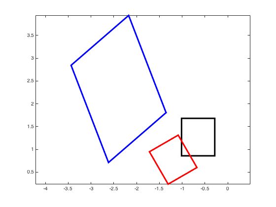
3 Let's get a visual intuition for the SVD
figure %Open a figure
%Every rectangle (and we will illustrate everything here with a rectangle
%can be defined by 4 numbers. The 4 numbers we will draw randomly
%here are x-position and y-position of corner, width and height
M = randn(1,4) %CornerX, CornerY, Width, Height
%Now, we need to translate that into an x- and y-trace and plot those
xTrace = [M(1,1), M(1,1)+M(1,3), M(1,1)+M(1,3), M(1,1), M(1,1)]
yTrace = [M(1,2), M(1,2), M(1,2) + M(1,4), M(1,2) + M(1,4), M(1,2)]
plot(xTrace,yTrace,'color','k','linewidth',3)
axis equal
shg

%After generating the original rectangle, we now rotate it
%Rotation is done by us through multiplication with orthogonal matrices
%Later, we'll use one coming out of the SVD
%Here, we'll use a designed one, so we can pick how much to rotate
theta = degToRad(-30); %30 degrees in radians
U = [cos(theta) sin(theta); -sin(theta) cos(theta)]; %Rotation matrix
%Put the traces into a matrix so we can apply the rotation at once
R(1,:) = xTrace;
R(2,:) = yTrace;
RR = U*R; %Matrix multiplication
hold on %I want to see it in terms of the old coordinate system
pause
plot(RR(1,:),RR(2,:),'color','r','linewidth',3)
S = [2 0; 0 3] %This will compress the first dimension by half and double the 2nd one
SRR = S*RR; %Applying a stretch to the rotated rectangle.
pause
plot(SRR(1,:),SRR(2,:),'color','b','linewidth',3)

%Exercise: Create a function where the user can input rotation angle,
%stretch factors (one for each dimension) and an arbitrary matrix and it
%outputs plots of the original matrix (rectangle) and the transformed one

%Add the 2nd rotation. We only did one.
M =
     -0.28529      0.85964     -0.72878      0.82052
xTrace =
     -0.28529      -1.0141      -1.0141     -0.28529     -0.28529
yTrace =
      0.85964      0.85964       1.6802       1.6802      0.85964
S =
     2     0
     0     3
4 Saving and loading
whos %Gives a list of variables in the workspace
save('MyFirstVariables') %This saves all variables. If you want to save only some, you need to list them by name
clear all %Delete everything in the workspace to show that the loading worked
whos
load('MyFirstVariables') %Load these variables again
%If these files are *not* in your working directory (or path), you need to
%give a path. Generally, we recommend to be in the path you need to be.
%You can do this programmatically with cd - change directory
  Name                         Size              Bytes  Class      Attributes

  A                      1000000x1             8000000  double
  B                       999996x1             7999968  double
  C                            2x2                  32  double
  D                            2x2                  32  double
  E                            1x1                   1  logical
  M                            1x4                  32  double
  R                            2x5                  80  double
  RR                           2x5                  80  double
  S                            2x2                  32  double
  SOP                          2x2                  32  double
  SRR                          2x5                  80  double
  U                            2x2                  32  double
  V                            2x2                  32  double
  ans                          2x2                   4  logical
  cumsum                       1x1                   8  double
  ii                           1x1                   8  double
  n                            1x50                400  double
  temp                    500499x1             4003992  double
  temp1                        1x50                400  double
  temp2                        1x50                400  double
  theta                        1x1                   8  double
  timeWithCommand              1x1                   8  double
  timeWithFind                 1x1                   8  double
  timeWithFunction             1x1                   8  double
  timeWithFunctions            1x1                   8  double
  timeWithLoop                 1x1                   8  double
  timeWithVector               1x1                   8  double
  x                            2x2                  32  double
  xTrace                       1x5                  40  double
  yTrace                       1x5                  40  double
5 Error checking and error correcting code
%This is a little bit of an advanced topic, but we'll do just enough of it
%for you to do the homework

A = randn(2,3)
B = randn(2,3)
%C = A*B %Where they touch, they need to match. Here, they don't, so MATLAB throws an error

%If MATLAB throws an error, execution of code is terminated. This can be
%problematic. It makes sense to write code in a flexible fashion. Basically
%anticipate that the user will do something ill-conceived and plan
%accordingly.

%MATLAB does this with try - catch statements

try %This is blue. This is recognized by MATLAB as a program flow command. It modifies the program flow
    C = A*B %Do the best you can to do it. Of course we know it will fail
catch %If you encounter an error in the course of programmatic affairs. By trying that.
    %Do this *instead* or *try this* instead
    %First thing: Tell the user that there was a problem
    disp('Error! You''re matrix dimensions did not match. That''s ok - we fixed that for you')
    C = A*B' %Transpose
end
A =
     -0.19824     -0.66304      -0.1039
      -1.1714       1.6994     0.073608
B =
        1.958      0.12326      0.81588
     -0.68751     -0.34372      0.19284
Error! You're matrix dimensions did not match. That's ok - we fixed that for you
C =
     -0.55463      0.34415
      -2.0241      0.23543
6 Vectorization
%MATLAB is optimized to handle matrices - as it is an interpreted
%language, loops will be slow. So, they should be avoided wherever
%possible. It is almost always possible. So why ever use loops? They do
%have their place - they always work and they are easy to understand.

%a) Creating a vector with a million elements
%First with a loop
clear A
tic %Starts the clock
for ii = 1:1e6
    A(ii,1) = ii; %Fill A from 1 to a million, via loop. Every time we go through it, we add a number
end
timeWithLoop = toc %Stops the stopwatch, and I want to save that number

%With a function
clear A
tic
A = linspace(1,1e6,1e6);
timeWithFunction = toc

%With a vector
clear A %Clear because I don't want to confer an unfair advantage to the vector
tic %Every time you call tick, a stopwatch is started
A = 1:1e6;
timeWithVector = toc %Every time you call toc, it is stopped

%Vector was ~200 times faster than the loop. This is typical
%Function was ~30 times faster.

%b) Checking whether elements are larger or smaller than some value
A = rand(1e6,1); %Matrix A with a million random numbers from 0 to 1
clear B %clear B to be fair
tic
for ii = 1:length(A) %Go through all elements of A
    if A(ii,1) > 0.5 %Check if it is larger or smaller than reference value
        B(ii,1) = 1; %If larger, assign 1 to appropriate spot in B
    else
        B(ii,1) = 0; %Otherwise zero
    end
end
timeWithLoop = toc

clear B
tic
B = A>0.5; %All at once
timeWithCommand = toc

clear B
tic
temp = find(A>0.5); %Use the find function to get the indices of the locations in A where the condition is true
B(temp(:,1),1) = 1; %Use these indices in B, setting them 1.
timeWithFind = toc

%Find is an amazing function. It doesn't give you values, it gives you the
%indices of the values where something you care about is true.

%Command was ~60 times faster than the loop
%Find was ~15 times faster than the loop
timeWithLoop =
      0.84983
timeWithFunction =
     0.011541
timeWithVector =
    0.0017938
timeWithLoop =
       1.4143
timeWithCommand =
   0.00097717
timeWithFind =
     0.016161
% c) Add only numbers in the vector that are large enough
%Now we combine these functions
A = rand(1e6,1); %Our random matrix with a million elements
cumsum = 0;
tic
for ii = 1:length(A) %Go through all elements of A
    if A(ii,1) > 0.5
        cumsum = cumsum + A(ii,1);
    end
end
cumsum
timeWithLoop = toc

%Version with find
tic
temp = find(A>0.5); %Just find the indices of those that are larger - ONE command, not a million
cumsum = sum(A(temp)) %Using these indices
timeWithFunctions = toc

%No difference in sum, but the functional way is ~75 times faster.

%Apart from speed, you can make sets nicely with vectors
%For instance
%Create a matrix of odd numbers from 1 to 100, their square roots and
%squares in 50 columns and 3 rows without a loop

format shortg %this avoids output in scientific notation
n = 1:2:100; %Every other one is an odd number
temp1 = sqrt(n); %Their square root
temp2 = n.^2; %Their square, element-wise
M = [n;temp1;temp2] %Stack the vectors to get a matrix
cumsum =
   3.7502e+05
timeWithLoop =
      0.99794
cumsum =
   3.7502e+05
timeWithFunctions =
     0.015579
M =
  Columns 1 through 6
            1            3            5            7            9           11
            1       1.7321       2.2361       2.6458            3       3.3166
            1            9           25           49           81          121
  Columns 7 through 12
           13           15           17           19           21           23
       3.6056        3.873       4.1231       4.3589       4.5826       4.7958
          169          225          289          361          441          529
  Columns 13 through 18
           25           27           29           31           33           35
            5       5.1962       5.3852       5.5678       5.7446       5.9161
          625          729          841          961         1089         1225
  Columns 19 through 24
           37           39           41           43           45           47
       6.0828        6.245       6.4031       6.5574       6.7082       6.8557
         1369         1521         1681         1849         2025         2209
  Columns 25 through 30
           49           51           53           55           57           59
            7       7.1414       7.2801       7.4162       7.5498       7.6811
         2401         2601         2809         3025         3249         3481
  Columns 31 through 36
           61           63           65           67           69           71
       7.8102       7.9373       8.0623       8.1854       8.3066       8.4261
         3721         3969         4225         4489         4761         5041
  Columns 37 through 42
           73           75           77           79           81           83
        8.544       8.6603        8.775       8.8882            9       9.1104
         5329         5625         5929         6241         6561         6889
  Columns 43 through 48
           85           87           89           91           93           95
       9.2195       9.3274        9.434       9.5394       9.6437       9.7468
         7225         7569         7921         8281         8649         9025
  Columns 49 through 50
           97           99
       9.8489       9.9499
         9409         9801