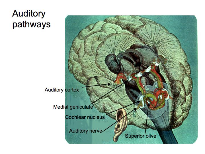
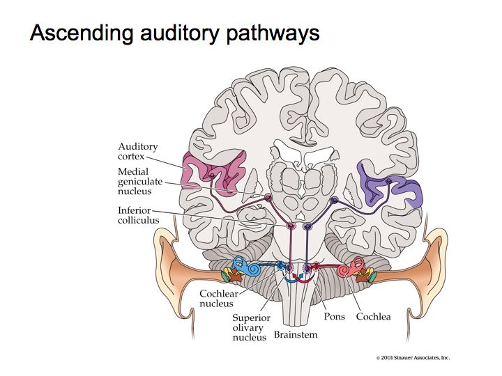
The primary auditory pathway begins with the auditory receptors in the cochlea. These synapse on spiking neurons in the spiral ganglia, the axons of which form the auditory (8th cranial) nerve. These then lead to the cochlear nucleus, then to the superior olive, then to the inferior colliculus, then to the medial geniculate nucleus, and finally on to auditory cortex.
Crossing of the Fibers. Significant number of nerve fibers cross the brain and make connections with neurons on the side opposite from the side of the ear in which they begin. This happens very early on in the auditory system. Inter-aural comparisons are an important source of information for the auditory system about where a sound came from (see spatial localization below).
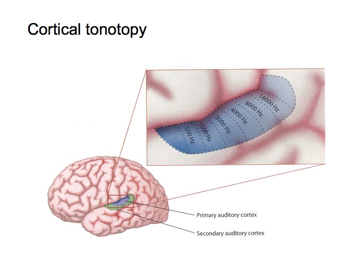
Tonotopic organization: The spatial layout of frequencies in the cochlea along the basilar membrane is repeated in other auditory areas in the brain. This is called tonotopic organization.
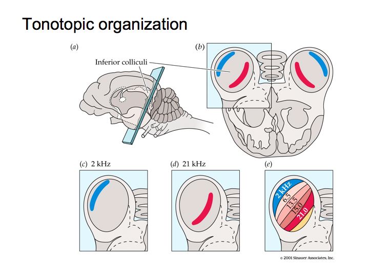
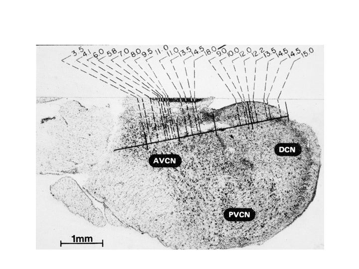
The figure above illustrates tonotonic organization in the inferior colliculus. The cochlear nucleus is also organized tonotopically. It has a couple of subregions or subnuclei. In each subnucleus (e.g., labelled AVCN and DCN in the figure below), nerve cells responsive to low frequencies are at one end and nerve cells that are responsive to high frequencies are at the opposite end, with the intervening frequencies laid out in their proper, ascending order.
Analogous tonotopic organization is also found in the auditory cortex.
Topographic maps of this sort are a big deal - we'll see many examples in the visual system of how information about various aspects of vision gets laid out amongst a collection of neurons in a systematic way.
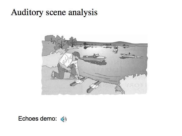
Al Bregman calls this the problem of auditory scene analysis and he uses this picture as an analogy for what your auditory system must do. The lake corresponds to your auditory world, the waves on the lake correspond to sound waves, the two channels correspond to your ear canals, and the two pieces of cloth correspond to your two ear drums. Just from the motion of the cloths, you have to figure out what's happening on the lake.
Auditory scene analysis is not all that well understood. But we do know that lots of things contribute to the perceptual organization (grouping or segregation) of sound signals. We often use auditory illusions to probe the organizational "rules" used by the auditory system (see the textbook for some examples of these "rules" of auditory perceptual organization).
One aspect of auditory scene analysis concerns echoes. In almost any room that you are in - but particularly a big room like our classroom - there are lots of echoes. And yet, we never seem to notice these echoes. Some of you may think that we don't notice the echoes because they are too weak, or inaudible. But that is not the case. In fact in the average room, 50 to 90 percent of the acoustic energy is reflected off the walls, and continues around the room, echoing for hundreds of milliseconds. In class we listened to a demonstration showing that in fact the echoes are quite strong - and quite audible - but that it is actually your brain that suppresses the naturally occurring echoes. The first part of the tape played the sound of a hammer striking a brick. Then, the sound was played backwards. The sounds were completely different in their apparent duration even though they were exactly the same sound, only played backwards in time. The reason for this is that the natural echoes in the environment are suppressed by your auditory system: they never reach your consciousness. It is only when we play the tape backwards so that the echoes arrive first that you can actually discern the enormous changes in the quality of the sound coming to you.
What's going on here? Let's say you clap your hands. I don't hear the distal stimulus, the physical event of clapping, directly. It's not like my head is sandwiched between your hands when you clap them. Rather, the physical event of clapping causes sound waves (changes in air pressure) that travel to my ears. Those sound waves also echo; they travel to the back of the room, bounce off the walls, and then on to my ears. The stimulus that reaches my ears is, therefore, a combination (a sum) of the sound wave that comes directly from your hands plus the sound waves that bounce around the room for a while before reaching my ears. The point is that my brain is not interested in the sound wave. If my hearing was sensitive to every echo of every noise, then things would obviously get very confusing. Rather, what's important is the physical event that gave rise to the sound wave. That's what I need to know about to survive and function in the world, whether the event was you clapping your hands or a tiger in the jungle stepping on a twig. So we don't hear (and most of the time we don't want to hear) a large portion of the physical stimulus (the sound waves) coming to our ears. And we're better off as a result. Our auditory system makes an unconscious inference from the sound wave to the physical event that caused the sound.
This is an excellent example of why we hear (and see) illusions. We don’t always sense things veridically, and we’re usually better off as a result. Our senses evolved to work as well as possible, subject to the limited information that they are provided. Most of the time this works out great, but sometimes your senses make obvious errors in the process of unconcious inference.
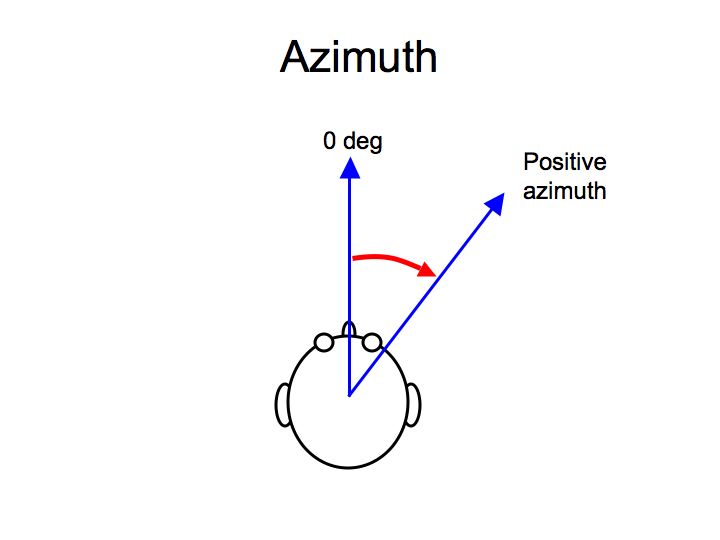
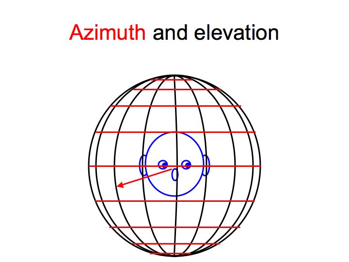
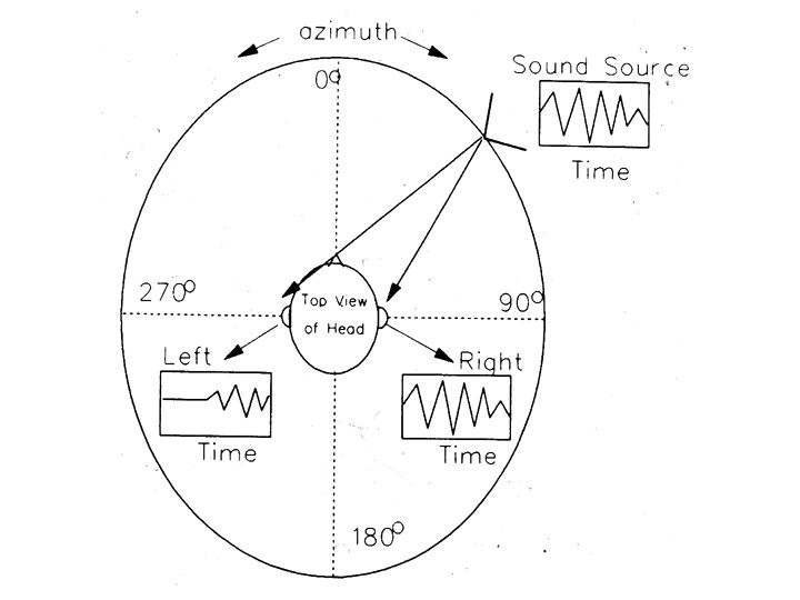
One sub-problem of auditory scene analysis is pretty well understood: spatial localization of sounds. Sounds can be localized using three coordinates: azimuth (the angle left or right of straight ahead), elevation (the angle above or below the horizontal plane) and distance.

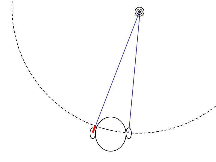
Two cues for localizing a sound source are: inter-aural intensity difference (IID) and inter-aural timing difference (ITD).
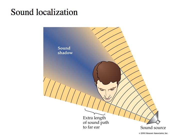
In above figures, the sound arriving at the ear that is furthest from the sound source is delayed (time difference) and lower in amplitude (intensity difference).
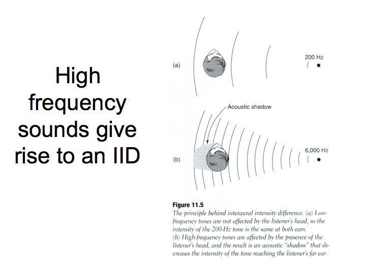
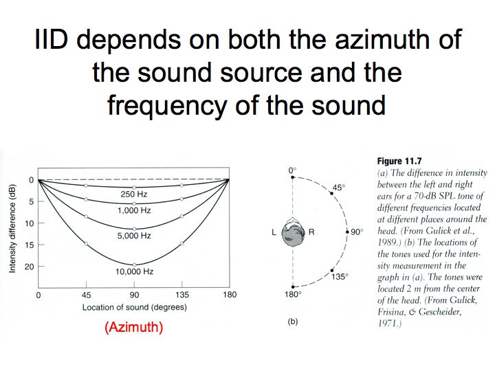
Intensity difference. If a sound is played at a position off to the right side, sound intensities will be slightly different in the two ears. First, the paths are of different length because sound has to travel past the head to get to the left ear and sound intensity decreases with distance (1/d2, where d is the distance to the sound source). Second, the head interferes with the sound-wave, casting the auditory equivalent of a shadow on the far ear. And, this sound shadow is more effective for sounds of higher frequency.
Timing difference. Sounds arriving from the right side also arrive at the right ear first because it's closer. This cue is especially easy to use with abrupt sounds, as you can compare the onset (beginning) of the sounds in each ear. For continuous pure tones, this is more difficult as it involves a phase difference between the sound in the two ears. This phase difference is ambiguous (is it 1/4 cycle, 1-and-1/4 cycles, or negative 3/4 cycles?), and the ambiguity can only be clearly resolved for lower frequencies.
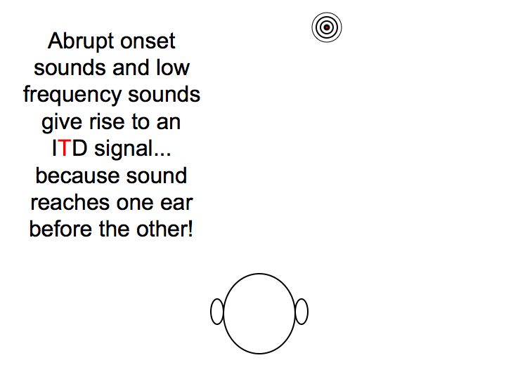
For the average person, the timing difference never exceeds .8 msec, i.e., very short. Indeed, this amount of time is actually smaller than the amount of time it takes to develop an action potential in the auditory nerve. Remarkably enough, this very precise temporal information is made available to your perceptual experience.
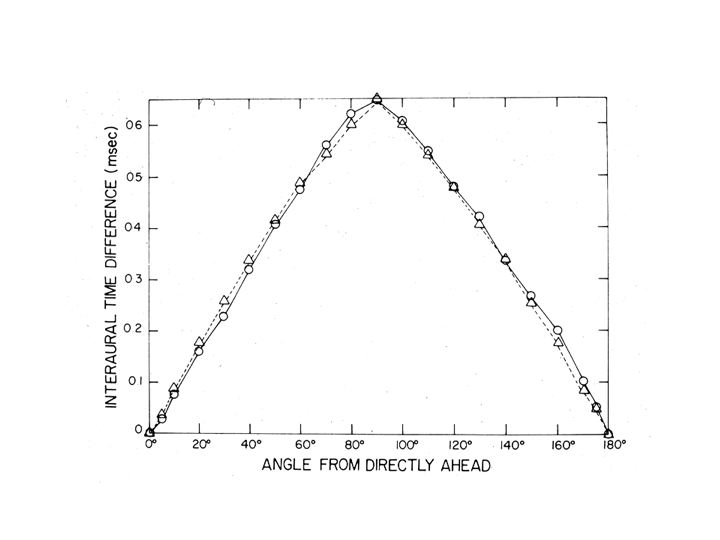
Measurements of timing differences
The two cues work together. Perceptual experiments conducted by Shaxby and Gage about 60 years ago examined these cues. They played two tones to the subject's two ears and set the timing between the two tones to be slightly different. A subject listening to these two tones with slightly different time delays hears a single tone. The position of the tone however is not directly in the middle of the head, but rather appears to be off to the side a bit. Then, they asked the subject to adjust the intensity of one of the two tones in order to make the tone seem to be positioned directly in the middle of the head. The subject was asked to make an intensity adjustment that would compensate - or balance - the adjustment that the experimenters imposed by the choice of inter-aural time delay.
The main result of this experiment is that subjects can do the task. That is, they can adjust the intensity of one of the tones and compensate for the time delay so that they hear but a single tone in the middle of their head. So, both cues (intensity difference and time delay) are combined to localize sound sources. A second important result is that the intensity difference needed to accomplish this is quite large. Very small differences in time between the two ears requires quite large differences in intensity to compensate for the perceived displacement of the sound.
Neurophysiological mechanisms of sound localization. Konishi (at CalTech) and his colleagues have performed a large number of auditory experiments on barn owls. While studying the inputs to the medial superior olive (MSO) and lateral superior olive (LSO), they discovered neural circuits and neurons that appear to be well-suited to representing these two types of information, both timing and intensity differences.
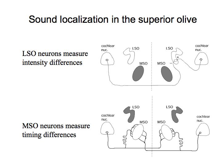
LSO contains neurons that are selective to intensity differences and MSO contains neurons that are selective for timing differences.
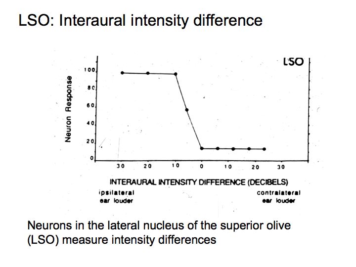
This graph shows the responses (firing rates) of an example LSO neuron that response strongly when the sound arriving at the ipsilateral ear is louder than the sound in the contralateral ear (Recall that there are two superior olives, one on the right and the other on the left, and note that ipsilateral means same side and contralateral means opposite side).
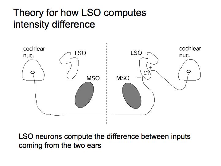
Let's say that the sound in the right ear is higher intensity than that in the left ear. Then the firing rates of neurons in the right cochlear nucleus are higher than those in the left cochlear nucleus. This hypothetical LSO neuron computes a difference between the firing rates (right cochlear nucleus firing rate minus left cochlear nucleus firing rate) and it responds strongly. Another LSO neuron does the opposite comparison (left minus right) and it would respond strongly only if the sound in the left ear is stronger than than in the right ear.

This graph shows the responses (firing rates) of an example MSO neuron to different interaural timing differences. It responds most strongly when the sound in the right ear leads that in the left ear by about 50 microseconds. There are other neurons in the MSO that respond best to different interaural timing differences. Some prefer it when the sound in the right ear leads and others prefer it when the sound in the left ear leads. Some neurons prefers 20 microseconds time lag. Others prefer 50 microseconds, 55 microseconds, 70 microseconds, 100 microseconds, 200 microseconds, etc. They work together to infer and represent the timing difference.
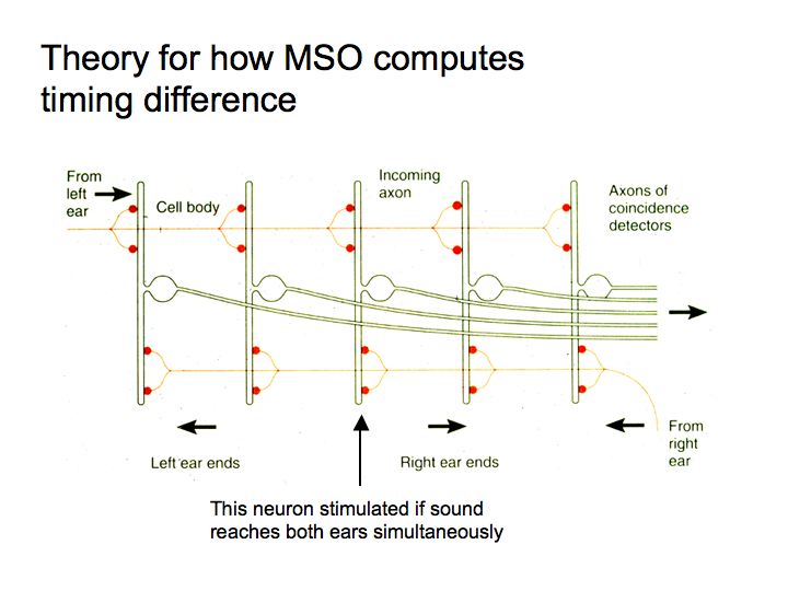
How do MSO neurons respond selectively to such short timing differences? Lloyd Jeffress, a psychophysicist, proposed a theory in the early 1950s. MSO neurons act as coincidence detectors. Coincident spikes arriving from the two ears evoke a response in the MSO neuron. Inputs from the two ears are delayed by various amounts relative to one another by the relative length of the axons. For this to work, the timing of individual spikes must be very precise, and it is, at least for low frequency tones because of phase locking.
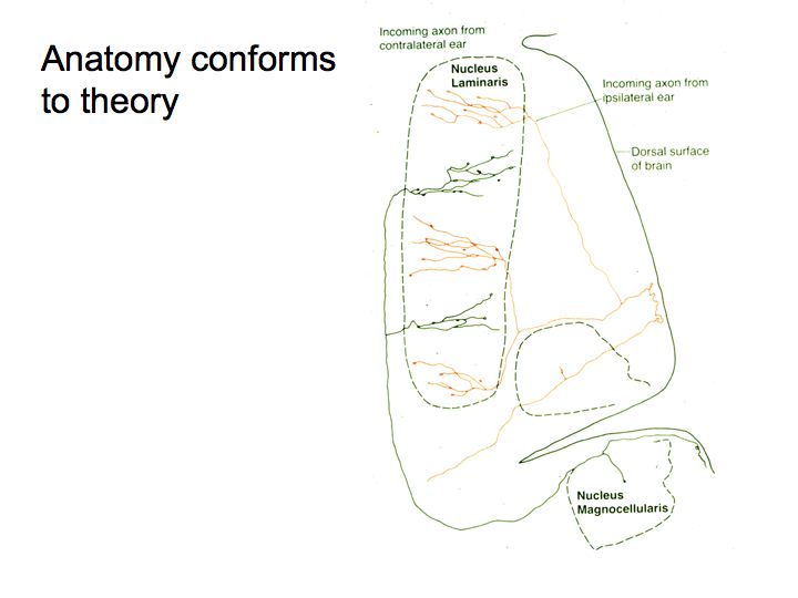
Konishi took a close look at the anatomy of the MSO (also called the nucleus laminaris) and found that the neurons are connected in a way that looks remarkably like the wiring diagram predicted by Jeffries. And, the temporal tuning of these nerve cells has precisely the property that Jeffress predicted. The neurons communicating signals from the two ears converge in a very orderly fashion, with increasing delay in the transmission length. The inputs from the two ears are combined to generate neurons whose preference for inter-aural time differences varies systematically.
The cone of confusion. Both the IID and ITD cues are based on a sound source being closer to one ear than the other. Geometrically, the set of locations in the world that are, say, 5 cm closer to one ear than the other is (approximately) a cone with its apex at the center of the head. Sound sources located at any position in the cone (above-right, in front and to the right, behind and to the right, closer, further) generate exactly the same IID and ITD cues for the listener and thus can not be distinguished using IIDs or ITDs. There are two ways to disambiguate the direction (azimuth and elevation) from which a sound is coming. (1) You can move and rotate your head. For example, if you move your head until the sound becomes maximally intense in one ear, then that ear must be pointed directly toward the sound (think of a cat or a dog orienting toward a sound by moving its head and/or ears). (2) The IID and ITD cues are, in fact, not identical from all points in the cone of confusion. The outer ears (the pinnae) are asymmetrically shaped, and filter sounds differently depending on where the sound sources are located and what frequency the sound has. If we measure the intensity of sounds at the ear drum as a function of their azimuth, elevation and frequency, the resulting data set is called the Head-Related Transfer Function (HRTF). This function describes the IID as a function of frequency by the attenuation characteristics, and the ITD as a function of frequency in the phase delay. When sounds are heard over headphones, they typically sound like the sound source is located inside the head. If the two ears' signals are first filtered using the listerener's HRTF, the sounds now are perceived as coming from outside the head. Thus, the differential filtering of sounds based on their frequency and location by the HRTF is a cue to sound location used by human observers.
Cues to distance. None of the cues described so far give any indication as to the distance to a sound source. A given sound source with a fixed physical intensity (at the source) results in a less intense signal (at the ear) as the distance to the source increases. Thus, intensity itself can be a cue to sound source distance. However, we also have a certain degree of loudness constancy (sounds appear equally loud as the sound source changes in distance, despite the change in intensity at the ear). Thus, there must be other cues to distance (as loudness constancy works, to some extent, even with your eyes closed). All sounds arrive at your ear both directly, and as echoes and reverberations involving reflections off the ground and other environmental surfaces. You normally don't perceive echoes as separate sounds (see above). However, the timing of these reflections and the number and intensity of them is a cue to the kind of space you are in (hallway, concert hall, living space, outdoors) and to the distance to the sound source.