
Behavioral Experiments: We need, in addition, to perform behavioral experiments. The goal is to interpret the brain activity in terms of perception and perceptually guided behavior. For example, what's the relationship between auditory nerve firing rates and perceived loudness or perceived pitch? What's the relationship between photoreceptor response and perceived brightness or perceived color?
The starting point for studying perception is to come up with a phenomenon. It might be an illusion... Or an observation (e.g., that we can localize sound sources by combining information between the two ears). Many of the basic phenomena in vision and hearing were discovered and described by Helmholtz in the late 19th century. For the last 100 years or so we have been trying and are still trying to explain those phenomena. Some perceptual scientists spend their entire careers coming up with new perceptual phenomena (illusions, etc.). This is more of an art than a scientific method, so I can't really tell you how to do it. But I will show you more examples of illusions, throughout the semester, some of which were discovered/created quite recently.
Ultimately, we want to establish a causal link demonstrating that a particular neural mechanism causes a particular perceptual phenomenon. To establish a strong link between perception and neurophysiology, we need to have quantitative measurements of both, and we need to show that they are consistent with one another. So next we will cover how we quantify perceptual phenomena.
There are three basic experimental protocols that we use in perceptual psychology experiments: magnitude estimation, matching and detection/discrimination.
Magnitude estimation: Subject rate (e.g., on a scale from 1-10) some aspect of a stimulus (e.g., how bright it appears or how loud it sounds).


Matching: In a matching experiment, the subject's task is to adjust one of two stimuli so that they look/sound the same in some respect. For example, you might adjust the intensity of two different tones so that they sound equally loud. Matching experiments are also sometimes done by presenting a series of trials and simply having the subject pick which trial had the best match. For example, each trial might consist of two tones and the subject picks the trial in which the tones sounded closest in loudness. There are other ways to do it as well, but they are all conceptually the same - find the stimulus conditions that look/sound the same in some respect (loudness, pitch, brightness, color, etc.). We'll see several examples of matching experiments later on in the course.

Detection/discrimination: In a detection experiment, the subject's task is detect small differences in the stimuli. Examples: detect whether or not a light was flashed, detect whether or not an auditory tone was played, discrimintate which of two stimuli is more intense, or report whether a chest X-ray does or does not show evidence of a lung tumor.

The method of adjustment: Ask observer to adjust the intensity of the light until they judge it to be just barely detectable. This is like what happens when you get fitted for a new prescription for eye glasses. Typically, the doctor drops in different lenses and asks you if this lens is better than that one.

Something is very unsatisfying about the method of adjustment: it is introspectionist/subjective. With this method, one is asking the observer to tell us what they think their own threshold is. When subjects are very inexperienced - and indeed, even when they are quite experienced - this can be a dangerous strategy. It is not so much that the subject is lying or being dishonest. Rather, it is simply difficult to judge when a light is on the threshold of visibility. Moreover, it's kind of stressful for the subject - does this lens work better or does that one work better?
Yes-No/method of constant stimuli: The observer is presented with a series of tones of various intensities. Each intensity is played several times (randomly intermixed). On each trial the observer is asked to report whether or not they heard it. We calculate the probability of detection (or percentage of "yes" responses) for each tone intensity. The data can then be plotted as follows:

Psychometric function: percentage of "yes" responses vs intensity
These curves are call psychometric functions; they plot the signal strength on the horizontal axis and the probability of the observer saying "Yes" on the vertical axis. The fifty percent point is commonly used as an estimate of threshold.
Why do the psychometric functions increase gradually with tone intensity? Discuss...
There's something seriously wrong here. All of the trials are signal trials. There are no catch trials (blanks, noise-alone trials). We only get hits and misses. We can make no estimate of false alarms. Signal detection theory tells us that we need to know both the hit rate and the false alarm rate to determine detectability. As a result, we cannot use the data from a yes-no experiment to estimate the sensitivity, d', separately from the observer's criterion.
Forced choice: This is the method we use most of the time. The signal is present on some trials; there is no signal on other trials ("catch trials"). The subject is forced to respond on every trial either ``Yes, the light was presented'' or ``No, it wasn't.'. If they're not sure then they must guess. With the forced-choice method, we have both types of trials (blank, noise-only trials some of the time and signal+noise trials at other times), so we can count both the number of hits and the number of false alarms to get an estimate of d'.

Demo of a forced choice experiment...
Two-interval forced choice: This is another method, elaborating the forced-choice method, that we use frequently. In this method, there are two stimuli presented (two "intervals"). They can be visual stimuli presented side-by-side, or they can be visual or auditory (or other) stimuli presented one after the other. One of the stimuli is a blank (noise-alone) and the other is a signal+noise stimuli (with an intensity that is typically randomly varied from trial to trial). The task is not to detect a signal as there is always a signal. Rather, the task is to indicate in which of the two intervals the signal occurred. Since there is always a signal, there is no need to correct for a bias to say "yes" (unlike the forced-choice, or signal detection paradigm). There may be an issue of a bias to choose one of the two intervals, however (e.g., the first one, or the one on the left).
Comparing the methods: Different experimental procedures lead to different estimates of threshold. For example, threshold settings from naive observers using the method of adjustment are usually about ten times higher than thresholds estimated by the forced choice procedure. With some practice this difference gets smaller. But even for experienced observers the adjustment thresholds and forced-choice thresholds are different by about a factor of 3.

Psychometric function: d' vs intensity
This function is also called a psychometric function, but it is slightly different from the psychometric functions plotted above for the yes-no method because this psychometric function plots d' on the vertical axis. The psychometric function starts at zero because if the subject is just guessing between the stimulus being presented or not s/he will have an equal number of false alarms and hits. Then d' rises with the test stimulus intensity. For a dim light there is a lot of overlap in the two (light off = noise only, light on = signal+noise) hypothetical distributions, so d' is small and it is hard to detect the light reliably. Note that we don't observe these internal responses directly. All we get is hit rate, false alarm rate, and d'. Small d' means that there must have been a lot of overlap in the hypothetical internal responses. When the light intensity is increased, discrimination is easier, hit rate goes up, false alarm rate goes down, d' goes up.
Choosing the threshold: We'll pick (more or less arbitrarily) a particular value of d' (we typically use d'=1 which corresponds to about 75% correct). The intensity that yields d'=1 performance is what we call threshold.
Discrimination: We can measure a threshold not only in the case when we are discriminating a signal from a no-signal stimulus, but also in the case when we are discriminating two signal levels from each other. Example: brightness difference threshold experiment where we ask the subject to identify which of two lights is the brighter one. On each trial we present either one light (with intensity x) or the other light (with intensity x+dx). The subject is forced to identify which of the two lights he or she thought was presented. And, we determine the smallest difference such that the two stimuli are just barely discriminable. We call this the difference threshold (or relative threshold). This is very similar to the absolute threshold case of the signal versus no-signal paradigm that we've been discussing up until now. In fact, the absolute threshold is really a special case when x is zero; we've been calling this a no-signal stimulus condition. So, the logic of the difference threshold experiment is no different from the logic of the absolute threshold experiment.

Let's say we measure brightness difference thresholds for a whole bunch of different base intensities. For each base intensity x we measure the intensity increment dx that is just detectable, collect up all the thresholds and graph them. Resulting data are very regular: dx is proportional to x. If we have a light of 10 units of intensity, dx needs to be about one unit of intensity. If we begin with 100 units of intensity then dx needs to be about 10 units of intensity, considerably larger than when we began with a light of only 10 units of intensity.
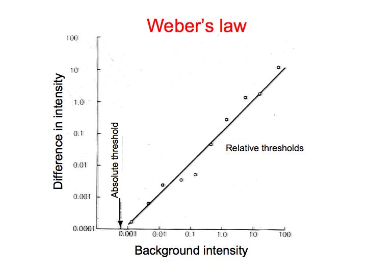
Generality of Weber's Law: These kinds of experiments have been performed in many different sensory modalities to measure our abilities to discriminate: intensities of 2 lights, intensities of two sounds, pressure on the skin, weight of two objects, intensity of electric shocks, and a whole host of other things. The result is always the same: The difference threhsold is proportional to the baseline/starting intensity. The generality of this observation proved so surprising that it has been called a psychological Law, and it is named after its discoverer, Weber. But it's not really a law per se (not like Newton's laws of motion, for example). Rather, it is an empirical observation, a phenomenon. Newton's laws in physics constitute a theory that explains a whole bunch of phenomena. Weber's law is just a description of the phenomenon itself. It wasn't until later that Fechner developed a hypothesis to explain Weber's observations.


Fechner's interpretation: Fechner had two key ideas. First, he came up with the idea of internal response that we've been relying on throughout this and the previous lecture. Second, Fechner hypothesized that when two signals are just noticeably different, it is as though they are separated by one unit of internal response.

On the horizontal axis we still have signal level, but now on the vertical axis we have units of psychological sensation (same as what we have been calling internal response). The threshold from a zero background to the first discriminable intensity level defines one unit of internal response. Then, starting at this new level, we can ask how much additional intensity do we need to reach a second unit of psychological sensation, and so forth. When you are done, you get a curve that relates a psychological quantity (internal response) to a physical quantity (stimulus intensity). As it turns out, the curve in this graph is logarithmic. So according to this graph, the internal response is predicted to be the logarithm of the stimulus intensity. Note that neither Weber nor Fechner measured the internal response directly. Fechner inferred something about the internal response (that it increases with the logarithm of stimulus intensity) from the behavioral threshold measurements. We can use this to make predictions about neurophysiology. Somewhere in the visual system, according to this analysis, there ought to be neurons that respond in proportion to the logarithm of stimulus intensity.
Weber-Fechner summary
Nowadays, nobody really believes Fechner's interpretation of Weber's law. The data are the same but the interpretation is different. It turns out that Weber's Law is also explained by assuming that the internal response is proportional to contrast, defined as the ratio of the intensity at a point divided by the local average intensity. Fechner's view has been substantially replaced by a hypothesis based on stimulus contrast. We'll talk more about contrast later in the semester.