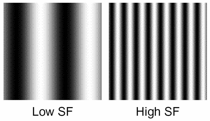
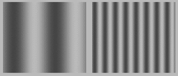
 Gratings with contrasts of 1 (top), .5
(middle) and 0 (bottom)
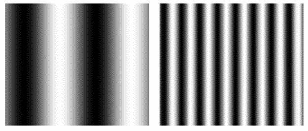
Gratings with contrasts of 1 (top), .5
(middle) and 0 (bottom)
The characterization of a system in linear systems theory is the
Modulation Transfer Function (MTF), i.e., the degree to which different
frequencies are amplified or attenuated by the system. The behavioral
analogy to the MTF is the
contrast
sensitivity function (CSF) which describes how sensitive an
observer is to sine wave gratings as a function of their spatial
frequency. This is measured using a contrast detection experiment
wherein one determines the minimum contrast required to detect sine
wave gratings of various spatial frequencies. As usual, sensitivity is
defined as 1/(threshold contrast) (so if threshold is low, sensitivity
is high).
 Sweep grating
The figure above shows a pattern that increases in spatial
frequency from left to right (the bars get narrower), and decreases in
contrast from bottom to top (the bars get fainter). By tracing out the
boundary between visible and invisible you can make out the curved
shape of your CSF. The typical results of such a measurement follow:
 Contrast sensitivity function
The typical CSF is bandpass in nature.
That is, you are most sensitive for an intermediate range of spatial
frequencies (around 4-6 cycles/degree), and less sensitive to spatial
frequencies both lower and higher than this, much like the audiogram.
The highest spatial frequency you can see (the
high frequency cutoff) determines
your spatial acuity, i.e., the finest spatial patterns you can see.
This acuity limit typically worsens with age.
Multiple spatial frequency channels
The CSF is typically not thought of as the MTF of a single kind of
neuron, but rather an envelope of sensitivity over several underlying
mechanisms, each corresponding to neurons with differing preferred
spatial frequencies (i.e., with different sizes of receptive field;
larger = lower spatial frequency preference). A graph illustrating this
follows:
In the figure above, four spatial frequency channels are illustrated,
and the notion is that the CSF represents the sensitivity pooled over
those underlying channels, i.e., sensitivity is primarily determined by
whatever channel (or set of neurons) is most sensitive to the stimulus.
Now, what does this parsing of the stimulus into different frequency
bands do for the observer?
Filtering
by spatial frequency channels - the neural image
As you can see, the low frequency filters provide information about
large objects, shadows, and other smooth, gradual changes in intensity
across the image. The higher spatial frequency filters emphasize
progressively finer details.
What evidence is there for the existence of multiple spatial frequency
channels? Well, first of all, there is the physiological evidence. In
V1 and beyond, for each location in the visual field there are neurons
varying in preferred spatial frequency, orientation, direction of
motion, and so on. But, there is behavioral evidence as well. First,
consider the effects of adapting to a particular spatial frequency. One
begins by measuring the CSF as illustrated in a figure above. Then, you
have the observer stare at a particular sine wave grating (e.g.,
8 cycles/degree) for an extended period of time. The visual system
adapts to that pattern, and
any neurons or mechanisms that were sensitive to that pattern become
desensitized temporarily. If one re-measures the CSF while in that
adapted state, the results are as follows:
The dotted curve represents the post-adaptation CSF and, as you can
see, sensitivity is reduced, but only for gratings with spatial
frequencies near that of the adapting grating. The idea is that the
spatial frequency channels sensitive to the adapting grating now have
reduced sensitivity due to all that stimulation, but those with spatial
frequency preferences distant from the adapter remain unaffected.
Spatial frequency adaptation not only affects threshold, but also
affects the appearance of supra-threshold gratings. After adaptation to
10 cycles/degree (i.e., even narrower bars), an 8 cycle/degree
grating will appear to have an even lower spatial frequency (even wider
bars). Likewise, after adapting to 6 cycles/degree (i.e., wider bars)
an 8 cycle/degree grating will appear to have an even higher spatial
frequency (even narrower bars). The explanation is illustrated here:
Explanation
of the size aftereffect
The idea is that adaptation to the higher spatial frequency
desensitizes the higher spatial frequency channels (those that "see"
the higher frequency grating). Then, when you display the 8
cycle/degree grating, the center of the response profile shifts to
lower frequencies (bottom-right graph above). When you adapt to a lower
spatial frequency grating, you see the opposite shift in the response
(upper-right graph). Similar shifts happen with orientation and
direction of motion, indicating that there are channels tuned for
various orientaitions and directions of motion.
There are two other common methods of demonstrating the existence of
multiple spatial frequency channels psychophysically. The first is
called
summation. There, the
idea is that if you ask an observer to detect a combination of two
grating (literally added together on the screen), the sensitivity is
much higher if the two gratings are close in spatial frequency (so that
they are detected by the same channel) than when they are far different
in spatial frequency (so that they are detected by separate channels).
A third psychophysical paradigm is called
masking. In this type of
experiment, the observer is asked to detect one
test grating (with frequency
f1) in the presence of another
masking grating (with frequency
f2). The masking grating is always
present, and the question is to what degree does it
mask the test grating, making it
harder to detect. It turns out that the results lead to the same model.
When the masking grating is similar in spatial frequency to the test
grating, masking is strong, and when it is dissimilar, masking is weak.
In other words, one grating masks another only to the extent that both
are detected by the same channel.